sponsors gamedev.net search:

Geo-morphing One problem with geometry management using level of detail is that at some point in time vertices will have to be removed or added, which leads to the already described "popping" effect. In our case of geo-mipmapping, where the number of vertices is doubled or halved at each tessellation level change, this popping becomes very visible. In order to reduce the popping effect geo-morphing is introduced. The aim of geo-morphing is to move (morph) vertices softly into their position in the next level before that next level is activated. If this is done perfectly no popping but only slightly moving vertices are observed by the user. Although this vertex moving looks a little bit strange if a very low detailed terrain mesh is used, it is still less annoying to the user than the popping effect. 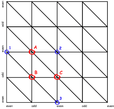It can be shown that only vertices which have odd indices inside a patch have to move and that those vertices on even positions can stay fixed because they are not removed when switching the next coarser tessellation level. Figure 6a shows the tessellation of a patch in tessellation level 2 from a top view. Figure 6b shows the next level of tessellation coarseness (level 3). Looking at Figure 6b it becomes obvious that the vertices '1', '2' and '3' do not have to move since they are still there in the next level. There are three possible cases, in which a vertex has to move: Case 'A': The vertex is on an odd x- and even y-position. This vertex has to move into the middle position between the next left ('1') and the right ('2') vertices. Case 'B': The vertex is on an odd x- and odd y-position. This vertex has to move into the middle position between the next top-left ('1') and the bottom-right ('3') vertices. Case 'C': The vertex is on an even x- and odd y-position. This vertex has to move into the middle position between the next top ('2') and the bottom ('3') vertices. Things become much clearer when taking a look at the result of the morphing process: after the morphing is done the patch is re-tessallated using the next tessellation level. Looking at Figure 6b it becomes obvious that the previously existing vertex 'A' had to move into the average middle position between the vertices '1' and '2' in order to be removed without popping. Figure 6a: Fine geometry with morphing vertices Figure 6b: Corresponding coarser tessellation level. Only odd indexed vertices were removed Optimizations Although the geometry's creation is very fast and we are rendering the mesh using only a small number of long triangle strips (usually about some hundred strips per frame), there are quite a lot of optimizations we can do to increase the performance on the side of the processor as well as the graphics card. As described in the section "Materials" we use a multi-pass rendering approach to apply more than one material to the ground. In the common case most materials will be used only in small parts of the landscape and be invisible in most others. The alpha-channel of the material's lightmap defines where which material is visible. Of course it's a waste of GPU bandwidth to render materials on patches which don't use that material all together (where the material's alpha channel is completely zero in the corresponding patch's part). It's easy to see, that if the part of a material's alpha-channel which covers one distinct patch is completely set to zero, then this patch does not need to be rendered with that material. Assuming that the materials' alpha channels won't change during runtime we can calculate for each patch which materials will be visible and which won't in a pre-processing step. Later at runtime, only those passes are rendered, which really contribute to the final image. Another important optimization is to reduce the number of patches which need to be rendered at all. This is done in three steps. First a rectangle which covers the projection of the viewing frustum onto the ground plane is calculated. All patches outside that rectangle will surely not be visible. All remaining patches are culled against the viewing frustum. To do this we clip the patches' bounding boxes against all six sides of the viewing frustum. All remaining patches are guaranteed to lie at least partially inside the camera's visible area. Nevertheless, not all of these remaining patches will necessarily be visible, because some of them will probably be hidden from other patches (e.g. a mountain). To optimize this case we can finally use a PVS (Potentially Visible Sets) algorithm to further reduce the number of patches needed to be rendered. 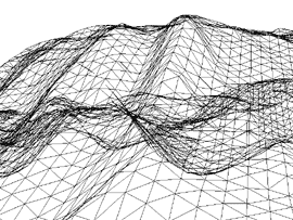PVS [Air91, Tel91] is used to determine, at runtime, which patches can be seen from a given position and which are hidden by other objects (in our case also patches). Depending on the type of landscape and the viewers position a lot of patches can be removed this way. In Figure 7 the camera is placed in a valley and looks at a hill. 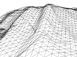Figure 7a: Final Image Figure 7b: Without PVS Figure 7c: With PVS Figure 7b shows that a lot of triangles are rendered which do not contribute to the final image, because they are hidden by the front triangles forming the hill. Figure 7c shows how PVS can successfully remove most of those triangles. The nice thing about PVS is that the cost of processing power is almost zero at runtime because most calculations are done offline when the terrain is designed. In order to (pre-) calculate a PVS the area of interest is divided into smaller parts. In our case it is obvious to use the patches for those parts. For example a landscape consisting of 16x16 patches requires 16x16 cells on the ground plane (z=0). To allow the camera to move up and down, it is necessary to have several layers of such cells. Tests have shown that 32 layers in a range of three times the height of the landscape are enough for fine graded PVS usage. One problem with PVS is the large amount of memory needed to store all the visibility data. In a landscape with 16x16 patches and 32 layers of PVS data we get 8192 PVS cells. For each cell we have to store which of all the 16x16 patches are visible from that cell. This means that we have to store more than two million values. Fortunately we only need to store one bit values (visible/not visible) and can save the PVS as a bit field which results in a 256Kbyte data file in this example case. 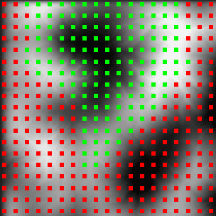Figure 8: PVS from Top View. Camera sits in the valley in the middle of the green dots Figure 8 shows an example image from the PVS calculation application where the camera is located in the center of the valley (black part in the middle of the green dots). All red dots resemble those patches, which are not visible from that location. Determining whether a patch is visible from a location is done by using an LOS (line of sight) algorithm which tracks a line from the viewer's position to the patch's position. If the line does not hit the landscape on its way to the patch then this patch is visible from that location. To optimize memory requirements the renderer distinguishes between patches which are active (currently visible) and those which aren't. Only those patches which are currently active are fully resident in memory. The memory footprint of inactive patches is rather low (about 200 bytes per patch). Geomorphing in Hardware

Contents   Introduction   Calculating the Tessellation Level of a Patch   Geo-morphing   Geomorphing in Hardware   Source code   Printable version   Discuss this article