Trees Part 2: Binary Trees
Click here to get the demo program and code samples.
I was talking to some people about ideas for this article, and when I proposed that it be about simple binary trees, someone said that games have no need for these, and that I should do something closer to game programming, such as BSP trees. I beg to differ here, actually. While the beginner may think that game programming is all about graphics, they are leaving out a critical part of the equation. Games these days are becoming incredibly large, and long dead are the days when a single hacker can throw together a game. It takes engineering skills and discipline, and most of all, an understanding in the basic concepts of data structures. Without knowing what data structures exist, and what they can do, how can anyone ever hope to make a large complex world that doesn’t choke the current line of computers? I feel that leaning about the basic data structures that have been developed and tested ever since computers were invented is an essential part of game programming. Indeed, what good is a carpenter who does not know how to use his tools? And now, without further ado, I give you part II of the Tree’s series.
Last time, we discussed recursion and the basic structure of trees. Now, I would like to get into an important sub-section of hierarchal data structures: Binary Trees. We all (hopefully) know that computers are binary machines, so it makes quite a bit of sense that the most frequently used kind of tree in computer programming is a binary tree. A Binary Tree is simply a tree in which every node has a maximum two children. Binary trees can be used for many things, such as efficient searching, arithmetic expression parsing, and data compression, etc. Before we get into the details, there are a few terms and definitions that need to be explained.
Algorithm Analysis and Big-O Notation
It is important to understand a little bit about how algorithms are rated for efficiency. Michael Abrash has said that "Without good design, good algorithms, and complete understanding of the program’s operation, your carefully optimized code will amount to one of mankinds least fruitful creations – a fast slow program," and he is absolutely correct. You can write the fastest code around, but if your algorithm is inherently slow, nothing will make it efficient. Big-O is a measure of the worst-case scenario (or complexity) of any given algorithm, as the size of the data set increases. It typically consists of an algebraic statement that represents the speed of the algorithm based on the size of the data it operates on. The Big-O of a sequential linked list search, for example, is O(n). Simply put, if you have n items, the worst case is that you would need to search through every item in the list, resulting in n comparisons. There are other Big-O cases, such as O(n^2), which is used to describe doubly nested for loop operations, or even O(2^n) or O(n!) (n-factorial, which is n*n-1*n-2*...3*2*1), which describe algorithms which take immense amounts of time to complete. The other two important worst-case scenarios are O(log n) and O(c), (where c is a constant value). In O(c), the algorithm completion time always takes the same amount of time to complete, no matter what size the data set is. This is used frequently to represent constant time algorithms, such as hash table lookups. O(log n) is the most important complexity when dealing with binary trees. If you don’t know what a logarithm is, don’t worry, it is not essential to the understanding of binary trees. All you need to know is what the graph of a logarithmic function looks like this:
In a base-2 logarithm, the y part of the graph only goes up by one whole integer every time the number of items in the data set (n) is doubled. If an algorithm can attain this level of complexity, it is usually considered pretty efficient. I will show you how to make an O(log n) search function using binary trees later on. Note: I have only dealt with base-2 logarithms here. Logarithms can exist for any base number, but they are not important in this article.
Binary Trees
As the name implies, a binary tree is simply a recursively-defined tree that can have a maximum of two children. The two children are commonly given the names left child and right child, and as I said in the last article, binary trees have an additional traversal called the in-depth traversal. Binary trees are used for many things, ranging from efficient searching techniques, data compression, and even arithmetic expression parsers (simple compilers). Note that some people refer to binary trees as ‘B-Trees’, which is incorrect! B-Trees are a special kind of multi-data per node tree used for advanced balancing algorithms, and Apple Macintoshes even use B-trees for their file systems. Be careful to not call a ‘Binary Tree’ a ‘B-Tree’! Before we discuss structure implementation strategies, there are a few properties that a binary tree can have which are important.
Properties of a Binary Tree
Since binary tree nodes can only have a maximum of two children, this fact introduces several properties that do not make sense on general trees. There are three important properties that a binary tree can have: fullness, balance, and leftness.
Fullness
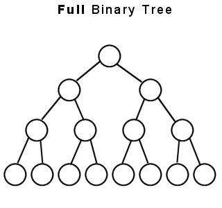
The first property is called fullness. A binary tree is considered full if, and only if, every node in the tree has either two or zero children, and every node which has zero children is on the lowest level of the tree. Because there is no limit to how many child nodes a general tree may contain, fullness of a general tree just doesn’t make sense, but any tree which has a limit on the number of children (ternary, quadnary, etc) can have this property.
Balance
The second property I’d like to discuss is balance. A binary tree can be balanced, such that one branch of the tree is about the same size and depth as the other. In order to find out if a tree node is balanced, you need to find out the maximum height level of both children in each node, and if they differ by more than one level, it is considered unbalanced. The easiest way to do this is to use a recursive function (the depth() function of the binary tree class which I have provided does this) to find the maximum depth of the left child, find the maximum depth of the right child, then subtract the two. If the number is –1, 0, or 1, the node is balanced. If the difference is anything else, then it is unbalanced. Note that a balanced binary tree requires every node in the tree to have the balanced property.
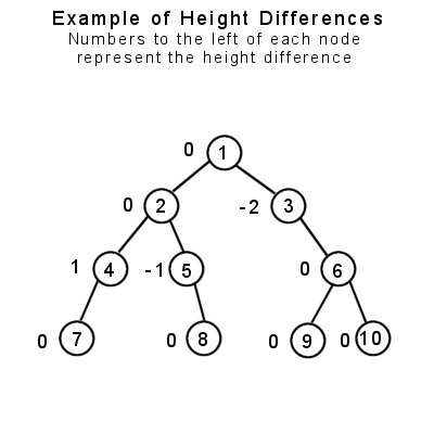
In this example, we see that the only node which is unbalanced is node #3, because the depth of its left side is 0, and the depth of the right side is 2. Subtracting 2 from 0 yields –2, thus that node is unbalanced. Note that node #1, the root, is considered balanced, since the maximum height level of both of its’ children is 3. This raises an important point: You cannot check just the root node for balancing, because it may be balanced but its child nodes may not be. Therefore, every node in the tree must be balanced in order for the tree to be considered balanced. The example tree above can be easily balanced by giving node #3 a left child.
Leftness
The third property I would like to discuss is leftness. This term is of my own creation, as I have never seen this term used before in textbooks, but it fairly important when dealing with some binary trees, such as Heaps. A leftist tree is basically a full tree, up until the lowest level. At the lowest level, every node does not need to be full, but it needs to fill in the leftmost part of the tree. While this is somewhat difficult to explain, a diagram helps immensely.
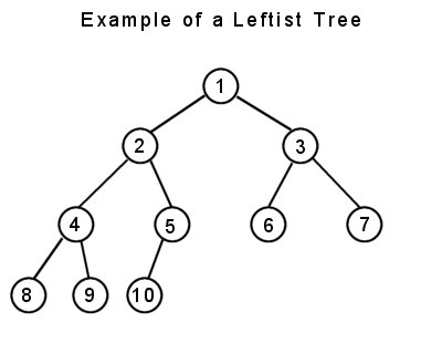
So, every child on the lowest level is pushed to the left of the tree. If you were to add one more node, it would need to be a right child of node #5 if the leftness property is to be maintained. This property becomes important when dealing with array-represented binary trees and heaps.
Structure Implementations of a Binary Tree
Linked Binary Trees
Binary Trees can be linked, just like the general tree was, where each node has two pointers to its children. This is the most common structure of binary trees.
General structure definition for a linked binary tree node:
template <class dataType>
class BinaryTree
{
public:
    typedef BinaryTree<dataType> node;
// --------------------------------------------------------------
//  Name:           BinaryTree::m_data
//  Description:    data stored in current tree node
// --------------------------------------------------------------
    dataType m_data;

// --------------------------------------------------------------
//  Name:           BinaryTree::m_parent
//  Description:    pointer to the parent of the node.
// --------------------------------------------------------------
    node* m_parent;

// --------------------------------------------------------------
//  Name:           BinaryTree::m_left
//  Description:    pointer to the left child of the node.
// --------------------------------------------------------------
    node* m_left;

// --------------------------------------------------------------
//  Name:           BinaryTree::m_right
//  Description:    pointer to the right child of the node.
// --------------------------------------------------------------
    node* m_right;
};
Notice how I made all the data public. While this destroys any semblance of good Object Oriented Design (OOD), there is a reason behind this. First of all, this is a tutorial on trees, not on object oriented design. If I were to go all out with OOD, I’d be using all sorts of esoteric features, totally eclipsing the theory behind the trees. Second, the binary tree node class is so simple, its definition is not likely to change anytime in the near future.
Advantages: the maximum tree size is limited only by the total memory available on the system.
Disadvantages: every tree node requires two pointers to its children, and this implementation uses a third for its parent. If only simple data types are being stored within the tree (integers, floats, characters), every node takes up 3-12 times the amount of space that the data type takes up.
Arrayed Binary Trees
There is one major variation of the structure of a binary tree: an arrayed binary tree. I have not implemented it here as an abstract data type, because its uses are fairly limited in the real world. However, I will implement a modified version for demonstrating heaps in the next tutorial. Right now, you should just know that the tree is represented as one large array:
It is traditional to represent arrayed nodes as boxes, rather than circles. This makes it easy to distinguish between the major structural differences. Note how the indexing starts at 1, and not 0. This is because of the rules that must be followed when traversing an arrayed binary tree:
The left child of any index i is at i * 2
The right child of any index i is at (i * 2) + 1
The parent of any index i is at i / 2 (integer division)
So, having an index of 0 would make traversal impossible. Take special care to note this fact: if node #2 does not exist within the tree, indices 2, 4, 5, 8, 9, 10, and 11 are all unusable, and therefore wasted. Also note that adding a right child to node #15 would increase the size of the array to 31 indices, of which #16 through #30 would not be used.
Advantages: Relatively fast to traverse, easy to transmit through serial interfaces (internet, external disk storage), saves much more space than a linked binary tree…
Disadvantages: but only if the tree is full, balanced, or leftist. Adding nodes to the tree that go beyond the capacity requires the array to be resized. Tree always has a size of (2d)-1, where d represents the maximum depth of any given node in the tree.
Methods of a Binary Tree
Here is a listing of all the methods in the binary tree class:
// ----------------------------------------------------------------
//  Name:           BinaryTree::BinaryTree
//  Description:    Default Constructor. Creates a tree node.
//  Arguments:      - data: data to initialize node with
//  Return Value:   None.
// ----------------------------------------------------------------
    BinaryTree( dataType p_data )

// ----------------------------------------------------------------
//  Name:           BinaryTree::~BinaryTree
//  Description:    Destructor. Deletes all child nodes.
//  Arguments:      None.
//  Return Value:   None.
// ----------------------------------------------------------------
    ~BinaryTree()

// ----------------------------------------------------------------
//  Name:           BinaryTree::setLeft
//  Description:    sets the left child pointer, rearranging parents
//                  as necessary. Existing left child is promoted
//                  to the root of its own tree, but beware, it is
//                  up to the client to remember where it is, or
//                  else there is a memory leak.
//  Arguments:      pointer to a binary tree node.
//  Return Value:   None.
// ----------------------------------------------------------------
    void setLeft( node* p_left )

// ----------------------------------------------------------------
//  Name:           BinaryTree::setRight
//  Description:    sets the right child pointer, rearranging parents
//                  as necessary. Existing right child is promoted
//                  to the root of its own tree, but beware, it is
//                  up to the client to remember where it is, or
//                  else there is a memory leak.
//  Arguments:      pointer to a binary tree node.
//  Return Value:   None.
// ----------------------------------------------------------------
    void setRight( node* p_right )

// ----------------------------------------------------------------
//  Name:           BinaryTree::preorder
//  Description:    processes the tree using a pre-order traversal
//  Arguments:      - process: A function which takes a reference
//                             to a dataType and performs an
//                             operation on it.
//  Return Value:   None.
// ----------------------------------------------------------------
    void preorder( void (*process)(dataType& item) )

// ----------------------------------------------------------------
//  Name:           BinaryTree::postorder
//  Description:    processes the tree using a post-order traversal
//  Arguments:      - process: A function which takes a reference
//                             to a dataType and performs an
//                             operation on it.
//  Return Value:   None.
// ----------------------------------------------------------------
    void postorder( void (*process)(dataType& item) )

// ----------------------------------------------------------------
//  Name:           BinaryTree::inorder
//  Description:    processes the tree using an in-order traversal
//  Arguments:      - process: A function which takes a reference
//                             to a dataType and performs an
//                             operation on it.
//  Return Value:   None.
// ----------------------------------------------------------------
    void inorder( void (*process)(dataType& item) )

// ----------------------------------------------------------------
//  Name:           BinaryTree::isLeft
//  Description:    determines if node is a left subtree. Note that
//                  a result of false does NOT mean that it is a
//                  right child; it may be a root instead.
//  Arguments:      None.
//  Return Value:   True or False.
// ----------------------------------------------------------------
    bool isLeft()

// ----------------------------------------------------------------
//  Name:           BinaryTree::isRight
//  Description:    determines if node is a right subtree. Note that
//                  a result of false does NOT mean that it is a
//                  left child; it may be a root instead.
//  Arguments:      None.
//  Return Value:   True or False.
// ----------------------------------------------------------------
    bool isRight()

// ----------------------------------------------------------------
//  Name:           BinaryTree::isRoot
//  Description:    determines if node is a root node.
//  Arguments:      None.
//  Return Value:   True or False.
// ----------------------------------------------------------------
    bool isRoot()

// ----------------------------------------------------------------
//  Name:           BinaryTree::count
//  Description:    recursively counts all children.
//  Arguments:      None.
//  Return Value:   the number of children.
// ----------------------------------------------------------------
    int count()

// ----------------------------------------------------------------
//  Name:           BinaryTree::depth
//  Description:    recursively determines the lowest relative
//                  depth of all its children.
//  Arguments:      None.
//  Return Value:   the lowest depth of the current node.
// ----------------------------------------------------------------
    int depth()
The setLeft/Right functions provide an easy way to set children in the tree. If a child already exists where you are inserting, it sets the existing child’s parent pointer to 0, making it a new tree. Then it puts the passed in node to whichever side you told it, and then sets the new nodes parent to the current node. All of this could be done manually, of course, but the method makes it simpler because that sequence of events happens quite frequently.
Next, I’ve added another traversal routine: inorder. I briefly touched on this in the last tutorial, so I’m going to explain it more in depth this time. An in-order traversal traverses the tree in this order:
- process left child
- process current data
- process right child
So the traversal only makes sense on binary trees, because it processes the current data in any given node between its two children.
isLeft/Right/Root should all make sense, they are just simple status functions.
count and depth are the two recursive status routines. As such, they should be used sparingly, because they are recalculated on each call. Count is simple to understand, it just recursively tells each of its children to return its count, adds one, and returns the result.
Depth is a bit more complex, as it takes the maximum of the relative depth of its left child and the relative depth of the right child, adds one and returns the result. The tree balancing routines discussed later on uses this method.
int depth()
{
    int left = -1;                    // clear left
    int right = -1;                   // and right
    if( m_left != 0 )                // if the left child exists
        left = m_left->depth();      // update the left depth
    if( m_right != 0 )               // if the right child exists
        right = m_right->depth();    // update the right depth
    if( left > right )               // if left is larger than
        return left + 1;             // right, return left + 1
    return right + 1;                // else return right + 1
}
Binary Search Trees
The most popular variation of the Binary Tree is the Binary Search Tree (BST). BSTs are used to quickly and efficiently search for an item in a collection. Say, for example, that you had a linked list of 1000 items, and you wanted to find if a single item exists within the list. You would be required to linearly look at every node starting from the beginning until you found it. If you're lucky, you might find it at the beginning of the list. However, it might also be at the end of the list, which means that you must search every item before it. This might not seem like such a big problem, especially nowadays with our super fast computers, but imagine if the list was much larger, and the search was repeated many times. Such searches frequently happen on web servers and huge databases, which makes the need for a much faster searching technique much more apparent. Binary Search Trees aim to Divide and Conquer the data, reducing the search time of the collection and making it several times faster than any linear sequential search.
Binary Search Tree Interface
Here is the general interface for a binary search tree. Notice that the BST class encapsulates binary tree nodes, rather than inherits them. This makes it easier to deal with a BST as one solid class, which handles insertions, searches and removals automatically for you.
// ----------------------------------------------------------------
//  Name:           BinarySearchTree::BinarySearchTree
//  Description:    Default Constructor. an empty BST
//  Arguments:      - compare: A function which compares two
//                             dataTypes and returns -1 if the left
//                             is "less than" the right, 0 if they
//                             are equal, and 1 if the left is
//                             "greater than" the right.
//  Return Value:   None.
// ----------------------------------------------------------------
    BinarySearchTree( int (*compare)(dataType& left, dataType& right) )

// ----------------------------------------------------------------
//  Name:           BinarySearchTree::~BinarySearchTree
//  Description:    Destructor.
//  Arguments:      None.
//  Return Value:   None.
// ----------------------------------------------------------------
    ~BinarySearchTree()

// ----------------------------------------------------------------
//  Name:           BinarySearchTree::insert
//  Description:    Inserts data into the BST
//  Arguments:      - p_data: data to insert
//  Return Value:   None.
// ----------------------------------------------------------------
    void insert( dataType p_data )

// ----------------------------------------------------------------
//  Name:           BinarySearchTree::has
//  Description:    finds the given data in the BST
//  Arguments:      - p_data: data to search for
//  Return Value:   true or false
// ----------------------------------------------------------------
    bool has( dataType p_data )

// ----------------------------------------------------------------
//  Name:           BinarySearchTree::get
//  Description:    finds the specified data within the tree and
//                  returns a pointer to it.
//  Arguments:      - p_data: data to search for
//  Return Value:   pointer to data, or 0 if not found.
// ----------------------------------------------------------------
    dataType* get( dataType p_data )

// ----------------------------------------------------------------
//  Name:           BinarySearchTree::remove
//  Description:    finds and removes data within the tree.
//  Arguments:      - p_data: data to find and remove
//  Return Value:   True if remove was successful, false if not.
// ----------------------------------------------------------------
    bool remove( dataType p_data )

// ----------------------------------------------------------------
//  Name:           BinarySearchTree::count
//  Description:    returns the count of items within the tree
//  Arguments:      None.
//  Return Value:   the number of items.
// ----------------------------------------------------------------
    inline int count()

// ----------------------------------------------------------------
//  Name:           BinarySearchTree::depth
//  Description:    returns the depth of the root node
//  Arguments:      None.
//  Return Value:   depth of the root node.
// ----------------------------------------------------------------
    inline int depth()

// ----------------------------------------------------------------
//  Name:           BinarySearchTree::inorder
//  Description:    processes the BST using an inorder traversal.
//  Arguments:      - process: A function which takes a reference
//                             to a dataType and performs an
//                             operation on it.
//  Return Value:   None.
// ----------------------------------------------------------------
    inline void inorder( void (*process)(dataType& item) )

// ----------------------------------------------------------------
//  Name:           BinarySearchTree::preorder
//  Description:    processes the BST using a preorder traversal.
//  Arguments:      - process: A function which takes a reference
//                             to a dataType and performs an
//                             operation on it.
//  Return Value:   None.
// ----------------------------------------------------------------
    inline void preorder( void (*process)(dataType& item) )

protected:
// ----------------------------------------------------------------
//  Name:           BinarySearchTree::find
//  Description:    finds a piece of data in the tree and returns
//                  a pointer to the node which contains a match,
//                  or 0 if no match is found.
//  Arguments:      - p_data: data to find
//  Return Value:   pointer to node which contains data, or 0.
// ----------------------------------------------------------------
    node* find( dataType p_data )

// ----------------------------------------------------------------
//  Name:           BinarySearchTree::removeNotFull
//  Description:    removes a node from the tree which has only one
//                  or no children.
//  Arguments:      - x: pointer to the node to remove
//  Return Value:   None.
// ----------------------------------------------------------------
    void removeNotFull( node* x )

// ----------------------------------------------------------------
//  Name:           BinarySearchTree::findLargestNode
//  Description:    finds the largest node in a subtree
//  Arguments:      - start: pointer to the node to start at
//  Return Value:   pointer to the largest node
// ----------------------------------------------------------------
node* findLargestNode( node* start )

// ----------------------------------------------------------------
//  Name:           BinarySearchTree::removeFull
//  Description:    removes a node from the tree which has two
//                  children
//  Arguments:      - x: pointer to the node to remove
//  Return Value:   None.
// ----------------------------------------------------------------
    void removeFull( node* x )
When constructing a BinarySearchTree, the constructor requires you to pass in a pointer to a comparison function. This function will be kept by the BST and invoked whenever the client inserts, searches for, or removes data. I have not allowed the client to modify the comparison function for a BST, simply because changing the comparison will ‘break’ the BST (see the section on BST validity below). The comparison works just like the standard C strcmp(), it takes two parameters, and compares them. If the left is ‘less than’ the right then it returns a negative value, If the left is ‘equal to’ the right it returns 0, and if the left is ‘greater than’ the right it returns a positive value. The actual meaning of the values are not important to the BST, it only cares if the value is 0, negative, or positive.
The basic operations are: insert, has, get, and remove. The algorithms for these will be discussed below. Along with these, there is a status method, count, which returns the current item count of the container, and inorder, which provides traversing capabilities to the BST by using an inorder recursive traversal, as described above. The preorder function is provided because the code prints out braces surrounding the children of each node, and gives a textual representation of the binary tree, allowing the client to see how the tree is actually constructed. The last four functions are all protected helper functions, and their usage and algorithms are also discussed below.
Validity of Binary Search Trees
The one rule that must always be followed for every node in a BST is this:
- the data element in the left subtree must be less than the value in the current node.
- the data element in the right subtree must be greater than the value in the current node.
If this rule applies to every node in a binary tree, then it is considered a valid Binary Search Tree. This is why changing the comparison function of the tree will break the tree; data to the left may not be less than data in the current node, etc.
Inserting Data
Inserting data into a binary search tree is a somewhat easy thing to do. The algorithm must follow the validity rules of a BST as stated above, and thus allows the client to insert data into the BST without being required to manually find the appropriate position. This is the main reason I chose to hide the underlying architecture of the binary tree and abstract it into a BST class. This is the general recursive algorithm for inserting data into a binary search tree node in pseudocode:
insert( dataType newData )
    if( newData < data )
        if( left != 0 )
            left.insert( newData );
        else
            left = new node( newData );
    else
        if( right != 0 )
            right.insert( newData );
        else
            right = new node( newData );
end insert
This routine follows the rules of a BST, and inserts the data to the left if it is less than the current data, and to the right if it is greater than the current data. The astute readers among you may have noticed something strange about the above: it breaks the second BST insertion rule just a tiny bit. If the new data is equal to the data already in the node, the algorithm inserts it to the right. Whether or not this is proper procedure, I’ll leave to the experts to decide. The benefit of this is that you can insert data and not have to worry about throwing an exception or returning an error value, but inserting data twice into a binary search tree does not make too much sense, because the search algorithm will never find subsequent instances of the data, unless the first instance is removed. Actual implementation, as always, is completely up to your needs.
One more important note about the above algorithm: While the provided algorithm is recursive, it doesn't need to be. Do you remember what I said in the first article, when I explained how recursion is great for implicitly keeping track of paths followed when traversing a tree? The insertion algorithm has no need to keep track of the path it travels, because once the new data is inserted, the algorithm can just stop execution immediately. I’ve re-written the algorithm to work without recursion:
void insert( dataType p_data )
{
    node* current = m_root;

    if( m_root == 0 )
        m_root = new node( p_data );
    else
    {
        while( current != 0 )
        {
            if( m_compare( p_data, current->m_data ) < 0 )
            {
                if( current->m_left == 0 )
                {
                    current->m_left = new node( p_data );
                    current->m_left->m_parent = current;
                    current = 0;
                }
                else
                    current = current->m_left;
            }
            else
            {
                if( current->m_right == 0 )
                {
                    current->m_right = new node( p_data );
                    current->m_right->m_parent = current;
                    current = 0;
                }
                else
                    current = current->m_right;
            }
        }
    }
    m_count++;
}
Notice how the iterative routine is more complex, but gets the job done quicker because it doesn’t need to travel back up the call stack after the node is actually inserted. Another important fact to note is that the node class needs to be modified to use the recursive function, while the iterative solution is best implemented as an external algorithm to the binary tree node. Since the BST class composes (as opposed to inheriting them) binary tree nodes, rather than modify the node class, the iterative solution is used instead in my provided code.
Building Binary Search Trees (examples)
Let's construct a few BSTs, shall we? Let's create a binary search tree with the data set: 50, 60, 40, 30, 20, 45, 65. (Diagram 1):
First, we start off with an empty tree, so 50 becomes the root node. We then insert 60, which is higher than 50, so we place it to the right of the root. In step 3, 40 is less than 50, so it goes to the left of the root. Since 30 is also less then 50, we try to insert it to the left of 50, but notice there is already a node there. So we go down one level and compare it to 40, and since 30 is less than 40 also, it goes to the left of that as well. In step 5, 20 goes to the left of 30, just like in step 4. In step 6, we insert 45. Since it is less than 50, it goes to the left of the root, but it is greater than 40, so we put it to the right of 40. Lastly, in step 7 we insert 65 to the right of 60. Note that this tree is considered height balanced.
Let's try another example. Insert 10, 20, 30, 40, and 50 into a new BST (Diagram 2):
Since every node is greater than the last, they all get added to the rightmost part of the tree. Notice what kind of structure this looks like: a linked list. A Binary Search Tree that doesn't branch is very inefficient for searching. It is not height balanced at all. We'll see how to optimize this kind of tree later on using AVL trees.
Finding Data In a Binary Search Tree
Now we get to the most important part of a BST: finding data within the tree (Really, what’s the point of a BST if you don't look for the data inside of it?). I am glad to say that finding data in a BST is very similar to inserting data. This also is best implemented as an iterative solution, since the algorithm has no need to travel back up the tree. I won’t even bother showing the recursive solution. The general algorithm for finding data is:
node* find( dataType p_data )
{
    node* current = m_root;
    int temp;

    while( current != 0 )
    {
        temp = m_compare( p_data, current->m_data );
        if( temp == 0 )
            return current;
        if( temp < 0 )
            current = current->m_left;
        else
            current = current->m_right;
    }
    return 0;
}
This algorithm shows the immense power of using a BST. Every time you compare a node and go down one level, the data left to search through is potentially halved. Divide and conquer indeed. I say ‘potentially’ because the number of data items is only halved when the tree is optimal, i.e. balanced. For our second BST building exercise, Diagram 2, there is absolutely no benefit of using the BST structure for searching. Let's look at Diagram 1, again. This time we want to find out if there is data within the tree. We'll look to see if it contains 45, 10, and 50.
Steps taken to search for 45:
- 45 is less than 50, so go down to the left
- 45 is greater than 40, so go down to the right
- 45 equals 45, so we found the node, return the node.
Steps taken to search for 10:
- 10 is less than 50, so go down to the left
- 10 is less than 40, so go down to the left
- 10 is less than 30, so go down to the left
- 10 is less than 20, but 20 has no left node, return 0.
Steps taken to search for 50:
- 50 equals 50, return the node.
The maximum number of comparisons needed to find any data in this tree is 4. Incidentally, a 4 level BST can contain a maximum of 15 data elements, and the log of 15 is 4 (actually it’s 3.9, but since we are dealing with discrete numbers, we need to take the ceiling of the function, and always round up if the number isn’t whole). Thus, we can double the number of elements in the tree to 31, but the number of comparisons required to find data in the tree only increases by 1, making 5 the maximum number of comparisons required by a balanced BST with 32 elements. This is why the optimal search time for a BST is considered O(log n).
However, there is one catch: the search algorithm for a binary search tree is actually considered O(n). How can this be? Remember, Big-O models the worst-case scenario of the algorithm, and if the tree looks like Diagram 2 above, then it is no more efficient than a linear search through a linked list. The AVL trees discussed in the next tutorial will remedy the situation.
Removing a node in a Binary Search Tree
In the general tree, we saw that removing a node from the tree also recursively removes all of its children, because it was assumed that the children were inherently related to the parent, and thus could not exist in the tree without the parent. A binary search tree is different, however, because of the way data is inserted. The user of the tree has no say in how the data is actually arranged within the tree, so it doesn’t make any sense for the tree to remove all the children of a single node when the user just wants to remove one data element from the tree. Thus, there is a special algorithm used to remove nodes from a binary search tree. The algorithm takes into account that the overall ordering of the tree needs to be maintained, and only manipulates pointers so that the removal is made quickly.
There are two cases when removing a node (call this node x) from a binary search tree:
- x has either one or no children.
- x has two children.
Case I: zero or one children
The first is the easiest to complete: the parent of x just needs to be told to point to the only valid child of x, or 0 if x has no children.
void removeNotFull( node* x )
{
    // find the valid child, or remain null if there
    // are no children.
    node* child = 0;
    if( x->m_left != 0 )
        child = x->m_left;
    if( x->m_right != 0 )
        child = x->m_right;

    if( x->isRoot() )
    {
        m_root = child;
    }
    else
    {
        if( x->isLeft() )
            x->m_parent->m_left = child;
        else
            x->m_parent->m_right = child;
    }

    // reset the parent node of the child, if it exists.
    if( child != 0 )
        child->m_parent = x->m_parent;

    x->m_left = 0;
    x->m_right = 0;
    delete x;
}
The function first finds out which child of x is valid. If neither of x’s children are valid, then the child variable remains null. Next, the algorithm determines what kind of node x is, whether it is the root, a left child, or a right child. Then the parent or the root is told to point to the determined child node. Lastly, x’s child pointers are cleared and it is deleted. It is imperative that the child pointers are cleared, because we are using a recursive node for this implementation which deletes all of its child nodes when deleted itself, and if its child pointers are not cleared, it will end up deleting nodes which should not be deleted.
Case II: two children
The second case is more difficult, because there are two nodes in the way, instead of just one. Now we must find a way to move up a node in one of the branches, so that the tree retains it’s ordering, and the node has only one child. Luckily for us, both the largest node and the smallest node in any given subtree are guaranteed to have only one or zero children. This is because of the BST validity rules: if the smallest node in a subtree had a left child, the child is larger than the smallest node, thus breaking the first BST rule. The same thing can be proved for the largest node in a subtree. Therefore, we have a choice, whether to move up the largest node from the left sub-tree to replace x, or the smallest node from the right sub-tree. For simplicity, I have elected to always choose the largest node in the left (call this node l), but take note that more optimized implementations may choose to determine which sub-tree is larger and then move the appropriate node up from there, in an effort to preserve the balancing of a tree.
The algorithm for finding the largest node in any given subtree is simple: travel down every right child of every node until you reach an empty right child. The first node with an empty right child will be the largest in the subtree. Here is the algorithm:
node* findLargestNode( node* start )
{
    node* l = start;

    // travel the path all the way down to the right.
    // the rightmost node is the largest in the subtree.
    while( l->m_right != 0 )
    {
        l = l->m_right;
    }
    return l;
}
There are two sub-cases when moving up the largest node in the left subtree:
- l is to the immediate left of x.
- l is hidden deeper in the left subtree of x.
In case 1, the parent of x needs to be changed to point directly to l. We can do this because we know that the largest node in any subtree will have no right children.
In case 2, the parent of x needs to be changed to point to l also, but there is a bit more work involved. We know that l is a right child of some other node now, and we also know that l has no right child, but l might have a left child. The solution is resolved exactly as if we were removing l from the tree (using a slightly modified removeNotFull() algorithm), by making the parent of l’s right pointer point to the left child of l. Then l’s left child needs to be changed to point to the left child of x, and l’s right child needs to be changed to point to the right child of x.
Nodes a and b do not necessarily exist, they could be null, or they could be valid, the algorithm works either way.
void removeFull( node* x )
{
    node* l = findLargestNode( x->m_left );

    // There are two cases:
    if( x->m_left == l )
    {
        // The largest node is immediately to the left
        // of the node to remove, so bypass x, and transfer
        // x's right child.
         l->m_right = x->m_right;
         l->m_right->m_parent = l;
    }
    else
    {
        // the largest node is somewhere deeper in the tree.
        // shortened removeNotFull algorithm <G>:
        // (notice how many assumptions can be made)
        l->m_parent->m_right = l->m_left;
        if( l->m_left != 0 )
            l->m_left->m_parent = l->m_parent;

        // now replace x with l.
        l->m_left = x->m_left;
        l->m_left->m_parent = l;
        l->m_right = x->m_right;
        l->m_right->m_parent = l;
    }

    if( x->isRoot() )
        m_root = l;
    else
    {
        if( x->isLeft() )
            x->m_parent->m_left = l;
        else
            x->m_parent->m_right = l;
    }

    l->m_parent = x->m_parent;
    x->m_left = 0;
    x->m_right = 0;
    delete x;
}
Removing Nodes from a Binary Search Tree (examples)
Now, we’re going to try removing some nodes from the tree. We’ll take the same diagram 1 that we built earlier, and remove 20, 60, and 50, in that order.
20 is easy to remove, as it is a leaf node. 30 is simply notified that it no longer has a left child. Removing 60 uses the same algorithm. Since it has only one child, 50’s right pointer is changed to bypass 60 and point directly to 65. Removing 50 is a bit more difficult, as it has two children. We need to find a node that has only one child and move it upwards. Since the algorithm we are using just finds the largest node in the left subtree, it decides to move 45 up into 50’s place.
Final note on the remove algorithm
I made this algorithm up myself. It is an extensive modification of the existing algorithms that I have found, which have all turned out to be inadequate. Most algorithms I have found use three or four cases, and separate the one or no child cases into separate algorithms. I condensed them into one algorithm, because they do the same thing. One algorithm I found even goes as far as finding the largest node in the left branch, whenever x has a left child, even if it doesn’t have a right child. This is clearly wasteful, because it could simply move the left child up one level, without having to search for the largest child in the subtree. Regardless, I am one hundred percent certain that the algorithm I have provided is flawless, I have done extensive testing, and formally written out every case possible on paper and solved them.
Sorting Data with a Binary Search Tree
One thing that I’ve always found cool about a binary search tree is that is automatically sorts data as it is inserted, with an algorithm whose optimal complexity is. If you look at what the actual tree looks like, it may not seem very sorted at first, but try tracing through an in-order traversal by hand. You’ll see that it actually traverses every item in the tree in order! Hence the name, in-order traversal. Try it on this tree:
An in-order traversal results in: 20, 30, 40, 45, 50, 60, 65. The optimal sorting time of a BST sort is approximately O(n log n), with a worst case of O(n2), which is in the same area of a quicksort and a heap sort, two of the most efficient sorts that exist.
Optional: Non-recursive Binary Tree techniques
I consider this section optional, and have included it only for completeness. It discusses ways in which binary tree traversals can be modified to make them iterative rather than recursive. A recent trend in the computer gaming industry is portability. While it is true that the Nintendo GameBoy is over ten years old, the market somewhat dried up within the past three years, but it has recently been warming up again. With powerful small devices such as the Cybiko becoming popular, handheld PDAs appearing everywhere, the not-so-distant release of the GameBoy Advance, and a thriving community of graphing calculator programmers, it is not surprising that portable games are also becoming popular. However, the public has been spoiled lately by all the 3d games, that a handheld game in today’s market really needs to fill some large shoes. Simple little games are not going to cut it anymore, and thus algorithms and data structures used to efficiently store huge worlds need to be created. This is where the iterative solutions come into play: All of these devices have horribly small stacks (compared to their big brothers, the PCs and game consoles), and will crash after a small number of function calls.
Let's get real for a moment though, shall we? If a handheld system has a small stack, it most likely has a small memory also. This makes binary trees a somewhat inappropriate choice of a data structure, simply because of the many links that need to be maintained, and waste memory. This is exactly why I consider this portion optional: I have not yet found a real-world use for non-recursive tree iterations that warrants the overhead of an iterative routine. The very fact that they can be made iterative, however, is a nice example of how every recursive algorithm can be made iterative, something Discrete Mathematicians like figuring out. <G>
Threaded Trees
Note that the term thread here has no relation to the name commonly given to computer processes. Thread, in this case, simply refers to a sewing analogy; essentially, every empty child pointer in the tree keeps a thread attached to the next node in an in-order traversal routine. I have actually implemented one of these before, as a project for school, and let me say this: I have absolutely no desire to ever work with one of these structures, ever again. While the theory behind it is simple, actual implementation is quite difficult, especially for the remove algorithm, which took 7 pages of code alone. Here’s a diagram:
Basically, the idea of a thread (the red lines) is to utilize the unused space of empty child pointers. So the thread pointers are exactly like normal child pointers, but they require a boolean to determine if the link is a thread or a child link. So each thread points to the next or previous node in an in-order traversal. Left threads point to the previous node, right threads point to the net node. Traversing this kind of tree requires some checks, and goes like this:
inOrder( process() )
    current = root;
    while( current.left != 0 )
        current = current.left

    while( current != 0 )
        process( current )
        if( current.hasRightThread() )
            current = current.right
        else
            current = current.right
            while( !current.hasLeftThread )
                current = current.left
            end while
        end if
    end while
I Just want to finish up by saying that while threads are a pretty cool idea, I honestly don’t think that the extra effort needed to rearrange the threads are worth the effort unless recursion as a solution is to be avoided at all costs.
Another in-order traversal method
Here is another technique for iteratively tracing through an in-order traversal. The basic idea operates on a few assumptions:
- When you are processing any node, the left child has already been processed, and the right child has not
- If the node being processed has no right child, and the current node is a left child, then the node above it has not been processed (think about it for a minute).
- If the node being processed has no right child, but the current node is a right child, then you need to travel up until you find a left child, then go up one more level.
It takes a fair amount of checking to remove the recursion, but if you cannot use recursion, the method is worth the extra effort:
inline void inorderIterative( void (*process)(dataType& item) )
{
    node* current;
    current = m_root;
    if( current != 0 )
    {
        while( current->m_left != 0 )
            current = current->m_left;
        while(1)
        {
            process( current->m_data );
            if( current->m_right != 0 )
            {
                current = current->m_right;
                while( current->m_left != 0 )
                    current = current->m_left;
            }
            else
            {
                if( current->isLeft() )
                {
                    current = current->m_parent;
                }
                else
                {
                    while( current->isRight() )
                        current = current->m_parent;
                    if( current->isRoot() )
                        return;
                    current = current->m_parent;
                }
            }
        }
    }
}
This assumes that the root node has a parent pointer of 0. And there you have it.
Conclusion
Well, I just looked at the page count, and I am up to 26 pages without the diagrams, which is somewhat larger than the first article. I did mean to get to three other types of trees in this article, but I think it’s better to put them in the next article, along with another type. The four I hope to discuss are:
- AVL Trees: These help the balancing problem that BSTs have when data is inserted in a somewhat ordered fashion.
- Splay Trees: These are BSTs which dynamically move data up to the top of the tree based on how frequently it is accessed. These help optimize searches on data sets that have locality-of-reference.
- Heaps: Another sorted tree structure, used in efficient priority queue implementations.
- Huffman Trees: Simple, yet elegant data compression.
Better to let all this sink in, before you go on to learning even more. I’m sorry I overestimated what I could reasonably fit into one article, but I promise I’ll get started on it immediately. So, the previously planned topics for Article #3 are now pushed back to a fourth article. Until next time!
Discuss this article in the forums
Date this article was posted to GameDev.net: 6/28/2001
(Note that this date does not necessarily correspond to the date the article was written)
See Also:
Data Structures
© 1999-2011 Gamedev.net. All rights reserved. Terms of Use Privacy Policy
Comments? Questions? Feedback? Click here!