Terrain Geomorphing in the Vertex Shader
The following article is an excerpt from ShaderX2 - Shader Programming Tips and Tricks, published by Wordware presumably in August 2003 (see www.shaderx2.com for more information).
Get the source code for this article here.
Introduction
Terrain rendering has heretofore been computed by a CPU and rendered by a combination of CPU and GPU. It is possible to implement a fast terrain renderer which works optimally with current 3D hardware. This is done by using geo-mipmapping which splits the terrain into a set of smaller meshes called patches. Each patch is triangulated view-dependently into one single triangle strip. Special care is taken to avoid gaps and t-vertices between neighboring patches. An arbitrary number of textures can be applied to the terrain which are combined using multiple alpha-blended rendering passes. Since the terrain's triangulation changes over time, vertex normals cannot be used for lighting. Instead a pre-calculated lightmap is used. In order to reduce popping when a patch switches between two tessellation levels geo-morphing is implemented. As will be pointed out later, this splitting of the terrain into small patches allows some very helpful optimizations.
Why geomorphing?
Terrain rendering has been an active research area for quite a long time. Although some impressive algorithms were developed, the game development community has community has rarely used these methods because of the high computational demands. Recently, another reason for not using the classic terrain rendering approaches such as ROAM [Duc97] or VDPM [Hop98] emerged: modern GPUs just don't like CPU generated dynamic vertex data. The game developers' solution for this problem was to build very low resolution maps and fine-tuned terrain layout for visibility optimization. In contrast to indoor levels, terrain visibility is more difficult to tune and there are cases where the level designer just wants to show distant views.
The solution to these problems is to introduce some kind of terrain-LOD (level of detail). The problem with simple LOD methods is that at the moment of adding or removing vertices, the mesh is changed which leads to very noticeable popping effects. The only clean way out of this is to introduce geomorphing which inserts new vertices along an existing edge and later on moves that vertex to its final position. As a consequence the terrain mesh is no longer static but changes ("morphs") every frame. It is obvious that this morphing has to be done in hardware in order to achieve a high performance.
Previous Work
A lot of work has already been done on rendering terrain meshes. Classic algorithms such as ROAM and VDPM attempt to generate triangulations which optimally adapt to terrain given as a heightmap. This definition of "optimally" was defined to be as few triangles as possible for a given quality criteria. While this was a desirable aim some years ago, things have changed.
Today the absolute number of triangles is not as important. As of 2003, games such as "Unreal 2" have been released which render up to 200000 triangles per frame. An attractive terrain triangulation takes some 10000 triangles. This means that it is no longer important if we need 10000 or 20000 triangles for the terrain mesh as long as it is done fast enough. Today "fast" also implies using as little CPU processing power as possible since in real life applications the CPU usually has more things to do than just drawing terrain (e.g. AI, physics, voice-over-ip compression, etc...). The other important thing today is to create the mesh in such a way that the graphics hardware can process it quickly, which usually means the creation of long triangle strips. Both requirements are mostly unfulfilled by the classic terrain meshing algorithms.
The work in this article is based on the idea of geo-mipmapping de Boer by [Boe00]. Another piece of work that uses the idea of splitting the terrain into a fixed set of small tiles is [Sno01], although the author does not write about popping effects or how to efficiently apply materials to the mesh.
Building the Mesh
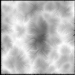
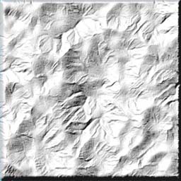
The terrain mesh is created from an 8-bit heightmap which has to be sized 2^n+1 * 2^n+1 (e.g. 17*17, 33*33, 65*65, etc�) in order to create n^2 * n^2 quads. The heightmap (see Figure 1a) can be created from real data (e.g. DEM) [Usg86] or by any program which can export into raw 8-bit heightmap data (e.g. Corel Bryce [Cor01]). The number of vertices of a patch changes during rendering (see view-dependent tessellation) which forbids using vertex normals for lighting. Therefore a lightmap (see Figure 1b) is used instead.
 |
 |
|
| Figure 1a: A sample heightmap | Figure 1b: Corresponding lightmap created with Wilbur |
In order to create the lightmap, the normals for each point in the heightmap have to be calculated first. This can be done by creating two 3d-vectors, each pointing from the current height value to the neighboring height positions. Calculating the cross product of these two vectors gives the current normal vector, which can be used to calculate a diffuse lighting value. To get better results, including static shadows, advanced terrain data editing software such as Wilbur [Slay95] or Corel Bryce should be used.
The heightmap is split into 17*17 values sized parts called patches. The borders of neighboring patches overlap by one value (e.g. value column 16 is shared by patch 0/0 and patch 1/0). Geometry for each patch is created at runtime as a single indexed triangle strip. A patch can create geometry in 5 different tessellation levels ranging from full geometry (2*16*16 triangles) down to a single flat quad (2 triangles, see Figure 2) for illustration. Where needed degenerate triangles are inserted to connect the sub-strips into one large strip [Eva96].
In order to connect two strips the last vertex of the first strip, and the first vertex of the second strip have to be inserted twice. The result is triangles which connect the two strips in the form of a line and are therefore invisible (unless rendered in wireframe mode). The advantage of connecting small strips to one larger strip is that less API calls are needed to draw the patch. Since index vertices are used and a lot of today's graphics hardware can recognize and automatically remove degenerate triangles the rendering and bandwidth overhead of the degenerate triangles is very low.
 |
| Figure 2: Same patch tessellated in different levels ranging from full geometry (level 0) to a single quad (level 4) |
Calculating the Tessellation Level of a Patch
Before a frame is rendered each patch is checked for its necessary tessellation level. It's easy to see from Figure 2 that the error of each patch increases as the number of vertices is reduced. In a pre-processing step, for each level the position of the vertex with the largest error (the one which has the largest distance to the corresponding correct position, later on called "maxerror vertex") is determined and saved together with the correct position.
When determining the level at which to render, all saved "maxerror vertices" are projected into the scene and the resulting errors calculated. Finally the level with the largest error below an application defined error bound is chosen. In order to create a specific level's geometry only the "necessary" vertices are written into the buffers. For example to create level 0 all vertices are used. Level 1 leaves out every second vertex reducing the triangle count by a quarter. Level 2 uses only every fourth vertex and so on�
Connecting Patches
If two neighboring patches with different tessellation levels were simply rendered one next to the other, gaps would occur (imagine drawing any of the patches in Figure 2 next to any other). Another problem are t-vertices, which occur when a vertex is positioned on the edge of an other triangle. Because of rounding errors, that vertex will not be exactly on the edge of the neighboring triangle and small gaps only a few pixels in size can become visible. Even worse, when moving the camera these gaps can emerge and disappear every frame which leads to a very annoying flickering effect.
To solve both problems it is obvious that each patch must know its neighbors' tessellation levels. To do so, all tessellation levels are calculated first without creating the resulting geometry and then each patch is informed about its neighbors' levels. After that each patch updates its geometry as necessary. Geometry updating has to be done only if the inner level or any of the neighbors' levels changed. To close gaps and prevent t-vertices between patches a border of "adapting triangles" is created which connects the differently sized triangles (see Figure 3). It is obvious that only one of two neighboring patches has to adapt to the other. As we will see later on in the section "Geomorphing", it is necessary for the patch with the finer tessellation level (having more geometry) to adapt.
 |
 |
|
| Figure 3a: T-vertices at the border of two patches | Figure 3b: T-vertices removed |
Figure 3a shows the typical case where T-vertices occur. In Figure 3b those "adapting triangles" at the left side of the right patch are created to avoid T-vertices. Although these triangles look like being a good candidate for being created by using triangle fans, they are also implemented using strips, since fans cannot be combined into bigger fans as can be achieved with strips.
Materials
Until now our terrain has no shading or materials yet. Applying dynamic light by using surface normals would be the easiest way to go, but would result in strange effects when patches switched tessellation levels. The reduction of vertices goes hand in hand with the loss of equal number of normals. When a normal is removed the resulting diffuse color value is removed too. The user notices such changes very easily - especially if the removed normal produced a color value which was very different from its neighboring color values.
The solution to this problem is easy and well known in today's computer graphics community. Instead of doing real time lighting we can use a pre-calculated lightmap which is by its nature more resistant to vertex removal than per-vertex lighting. Besides solving our tessellation problem, it provides us with the possibility to pre-calculate shadows into the lightmap. The disadvantage of using lightmaps is that the light's position is now fixed to the position that was used during the lightmap's generation.
In order to apply a lightmap (see Figure 4) we need to add texture coordinates to the vertices. Since there is only one lightmap which is used for the whole terrain, it simply spans the texture coordinates from (0,0) to (1,1).
 |
 |
|
| Figure 4a: Lit terrain | Figure 4b: Same terrain with wireframe overlay |
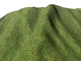
Now that the terrain's mesh is set up and shaded, it's time to apply some materials. In contrast to the lightmap we need far more detail for materials such as grass, mud or stone to look good. The texture won't be large enough to cover the complete landscape and look good, regardless of how high the resolution of a texture might be. For example if we stretch one texture of grass over a complete terrain one wouldn't even recognize the grass. One way to overcome this problem is to repeat material textures.
To achieve this we scale and wrap the texture so that it is repeated over the terrain. Setting a texture matrix we can use the same texture coordinates for the materials as for the lightmap. As we will see later this one set of (never changing) texture coordinates together with some texture matrices is sufficient for an arbitrary number of materials (each one having its own scaling factor and/or rotation) and even for moving faked cloud shadows (see below).
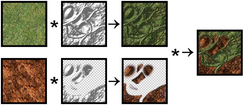
To combine a material with the lightmap two texture stages are set up using modulation (component wise multiplication). The result is written into the graphics buffer. In order to use more than one material, each material is combined with a different lightmap containing a different alpha channel. Although this would allow each material to use different color values for the lightmap too, in practice this makes hardly any sense. This results in one render pass per material which is alpha blended into the frame buffer. As we will see later a lot of fillrate can be saved if not every patch uses every material - which is the usual case (see section Optimization). Figure 5 shows how two materials are combined with lightmaps and then blended using an alpha map. (For better visualization the materials' textures are not repeated in Figure 5)
 |
| Figure 5: Combining two render passes |
In the top row of Figure 5 the base material is combined with the base lightmap. Since there is nothing to be drawn before this pass, no alphamap is needed. In the bottom row the second pass is combined with another lightmap. This time there is an alpha channel (invisible parts are drawn with checker boxes). The resulting image is finally alpha-blended to the first pass (right image in Figure 5).
It is important to note that this method allows each material pass to use a free scaling (repeating) factor for the color values which results in highly detailed materials while the lightmap does not need to be repeated since lighting values do not need as much detail. Only two texture stages are used at once, which allows combining an arbitrary number of passes. Most applications will not need more than three or four materials.
After all materials have been rendered, another pass can be drawn in order to simulate cloud shadows. Again we can repeat the shadows in order to get more detailed looking shadows. As we are already using a texture matrix to do scaling, we can animate the clouds easily by applying velocity to the matrix's translation values. The effect is that the clouds' shadows move along the surface which makes the whole scene looking far more realistic and "alive".
Geo-morphing
One problem with geometry management using level of detail is that at some point in time vertices will have to be removed or added, which leads to the already described "popping" effect. In our case of geo-mipmapping, where the number of vertices is doubled or halved at each tessellation level change, this popping becomes very visible. In order to reduce the popping effect geo-morphing is introduced. The aim of geo-morphing is to move (morph) vertices softly into their position in the next level before that next level is activated. If this is done perfectly no popping but only slightly moving vertices are observed by the user. Although this vertex moving looks a little bit strange if a very low detailed terrain mesh is used, it is still less annoying to the user than the popping effect.
It can be shown that only vertices which have odd indices inside a patch have to move and that those vertices on even positions can stay fixed because they are not removed when switching the next coarser tessellation level. Figure 6a shows the tessellation of a patch in tessellation level 2 from a top view. Figure 6b shows the next level of tessellation coarseness (level 3). Looking at Figure 6b it becomes obvious that the vertices '1', '2' and '3' do not have to move since they are still there in the next level. There are three possible cases, in which a vertex has to move:
- Case 'A': The vertex is on an odd x- and even y-position.
This vertex has to move into the middle position between the next left ('1') and the right ('2') vertices. - Case 'B': The vertex is on an odd x- and odd y-position.
This vertex has to move into the middle position between the next top-left ('1') and the bottom-right ('3') vertices. - Case 'C': The vertex is on an even x- and odd y-position.
This vertex has to move into the middle position between the next top ('2') and the bottom ('3') vertices.
Things become much clearer when taking a look at the result of the morphing process: after the morphing is done the patch is re-tessallated using the next tessellation level. Looking at Figure 6b it becomes obvious that the previously existing vertex 'A' had to move into the average middle position between the vertices '1' and '2' in order to be removed without popping.
 |
 |
|
| Figure 6a: Fine geometry with morphing vertices | Figure 6b: Corresponding coarser tessellation level. Only odd indexed vertices were removed |
Optimizations
Although the geometry's creation is very fast and we are rendering the mesh using only a small number of long triangle strips (usually about some hundred strips per frame), there are quite a lot of optimizations we can do to increase the performance on the side of the processor as well as the graphics card.
As described in the section "Materials" we use a multi-pass rendering approach to apply more than one material to the ground. In the common case most materials will be used only in small parts of the landscape and be invisible in most others. The alpha-channel of the material's lightmap defines where which material is visible. Of course it's a waste of GPU bandwidth to render materials on patches which don't use that material all together (where the material's alpha channel is completely zero in the corresponding patch's part).
It's easy to see, that if the part of a material's alpha-channel which covers one distinct patch is completely set to zero, then this patch does not need to be rendered with that material. Assuming that the materials' alpha channels won't change during runtime we can calculate for each patch which materials will be visible and which won't in a pre-processing step. Later at runtime, only those passes are rendered, which really contribute to the final image.
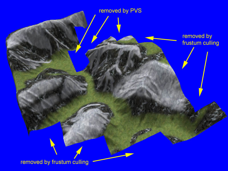
Another important optimization is to reduce the number of patches which need to be rendered at all. This is done in three steps. First a rectangle which covers the projection of the viewing frustum onto the ground plane is calculated. All patches outside that rectangle will surely not be visible. All remaining patches are culled against the viewing frustum. To do this we clip the patches' bounding boxes against all six sides of the viewing frustum. All remaining patches are guaranteed to lie at least partially inside the camera's visible area. Nevertheless, not all of these remaining patches will necessarily be visible, because some of them will probably be hidden from other patches (e.g. a mountain). To optimize this case we can finally use a PVS (Potentially Visible Sets) algorithm to further reduce the number of patches needed to be rendered.
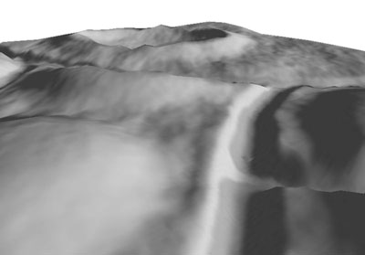
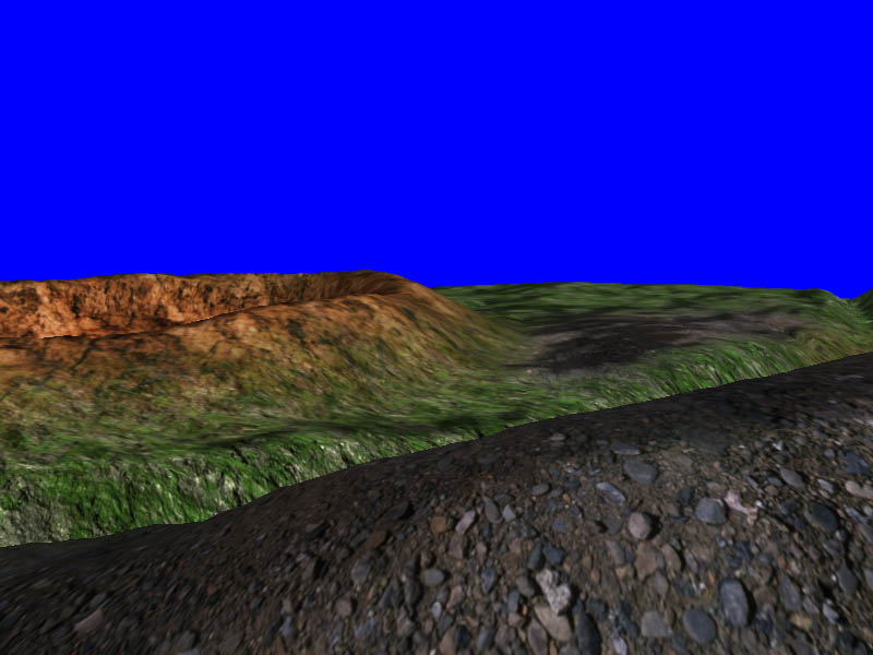
PVS [Air91, Tel91] is used to determine, at runtime, which patches can be seen from a given position and which are hidden by other objects (in our case also patches). Depending on the type of landscape and the viewers position a lot of patches can be removed this way. In Figure 7 the camera is placed in a valley and looks at a hill.
 |
 |
 |
||
| Figure 7a: Final Image | Figure 7b: Without PVS | Figure 7c: With PVS |
Figure 7b shows that a lot of triangles are rendered which do not contribute to the final image, because they are hidden by the front triangles forming the hill. Figure 7c shows how PVS can successfully remove most of those triangles. The nice thing about PVS is that the cost of processing power is almost zero at runtime because most calculations are done offline when the terrain is designed.
In order to (pre-) calculate a PVS the area of interest is divided into smaller parts. In our case it is obvious to use the patches for those parts. For example a landscape consisting of 16x16 patches requires 16x16 cells on the ground plane (z=0). To allow the camera to move up and down, it is necessary to have several layers of such cells. Tests have shown that 32 layers in a range of three times the height of the landscape are enough for fine graded PVS usage.
One problem with PVS is the large amount of memory needed to store all the visibility data. In a landscape with 16x16 patches and 32 layers of PVS data we get 8192 PVS cells. For each cell we have to store which of all the 16x16 patches are visible from that cell. This means that we have to store more than two million values. Fortunately we only need to store one bit values (visible/not visible) and can save the PVS as a bit field which results in a 256Kbyte data file in this example case.
 |
| Figure 8: PVS from Top View. Camera sits in the valley in the middle of the green dots |
Figure 8 shows an example image from the PVS calculation application where the camera is located in the center of the valley (black part in the middle of the green dots). All red dots resemble those patches, which are not visible from that location. Determining whether a patch is visible from a location is done by using an LOS (line of sight) algorithm which tracks a line from the viewer's position to the patch's position. If the line does not hit the landscape on its way to the patch then this patch is visible from that location.
To optimize memory requirements the renderer distinguishes between patches which are active (currently visible) and those which aren't. Only those patches which are currently active are fully resident in memory. The memory footprint of inactive patches is rather low (about 200 bytes per patch).
Geomorphing in Hardware
Doing geomorphing for a single patch basically means doing vertex tweening between the current tessellation level and the next finer one. The tessellation level calculation returns a tessellation factor in form of a floating point value where the integer part means the current level and the fractional part denotes the tweening factor. E.g. a factor of 2.46 means that tweening is done between levels 2 and 3 and the tweening factor is 0.46. Tweening between two mesh representations is a well known technique in computer graphics and easily allows an implementation of morphing for one single patch (vertices that should not move simply have the same position in both representations).
The problem becomes more difficult if a patch's neighbors are considered. Problems start with the shared border vertices which can only follow one of the two patches but not both (unless we accept gaps). As a consequence one patch has to adapt its border vertices to those of its neighbor. In order to do correct geomorphing it is necessary that the finer patch allows the coarser one to dictate the border vertices' position. This means that we do not only have to care about one tweening factor as in the single patch case but have to add four more factors for the four shared neighbor vertices. Since the vertex shader can not distinguish between interior and border vertices these five factors have to be applied to all vertices of a patch. So we are doing a tweening between five meshes.
As if this wasn't already enough, we also have to take special care of the inner neighbor vertices of the border vertices. Unfortunately these vertices also need their own tweening factor in order to allow correct vertex insertion (when switching to a finer tessellation level). To point out this quite complicated situation more clearly we go back to the example of figure 6b. For example we state that the patch's left border follows its coarser left neighbor. Then the tweening factor of vertex '1' is depends on the left neighbor, whereas the tweening factor of all interior vertices (such as vertex '2') depend on the patch itself. When the patch reaches its next finer tessellation level (figure 6a), the new vertex 'A' is inserted. Figure 9 shows the range in which the vertices '1' and '2' can move and the - in this area lying - range in which vertex 'A' has to be inserted. (Recall that a newly inserted vertex must always lie in the middle of its preexisting neighbors). To make it clear why vertex 'A' needs its own tweening factor suppose that the vertices '1' and '2' are both at their bottom position when 'A' is inserted (tweeningL and tweeningI are both 0.0). Later on when 'A' is removed the vertices '1' and '2' might lie somewhere else and 'A' would now probably not lie in the middle between those two if it had the same tweening factor as vertex '1' or vertex '2'. The consequence is that vertex 'A' must have a tweening factor (tweeningA) which depends on both the factor of vertex '1' (tweeningL - the factor from the left neighboring patch) and on that of vertex '2' (tweeningI - the factor by that all interior vertices are tweened).
 |
| Figure 9: Vertex insertion/removal range |
What we want is the following:
Vertex 'A' should
- be inserted/removed in the middle between the positions of Vertex '1' and Vertex '2'
- not pop when the patch switches to another tessellation level
- not pop when the left neighbor switches to another tessellation level.
The simple formula tweeningA = (1.0-tweeningL) * tweeningI does the job. Each side of a patch has such a 'tweeningA' which results in four additional tessellation levels.
Summing this up we result in having have 9 tessellation levels which must all be combined every frame for each vertex. What we actually do in order to calculate the final position of a vertex is the following:
PosFinal = PosBase + tweeningI*dI + tweeningL*dL + tweeningR*dR + tweeningT*dT + �
Since we only morph in one direction (as there is no reason to morph other than up/down in a heightmap generated terrain) this results in nine multiplications and nine additions just for the geomorphing task (not taking into account any matrix multiplications for transformation). This would be quite slow in terms of performance doing it on the CPU. Fortunately the GPU provides us with an ideal operation for our problem. The vertex shader command dp4 can multiply four values with four other values and sum the products up in just one instruction. This allows us to do all these calculations in just five instructions which is only slightly more than a single 4x4 matrix multiplication takes.
The following code snippet shows the vertex data and constants layout that is pushed onto the graphics card.
; Constants specified by the app
;
;    c0      = (factorSelf, 0.0f, 0.5f, 1.0f)
;    c2      = (factorLeft, factorLeft2, factorRight, factorRight2),
;    c3      = (factorBottom, factorBottom2, factorTop, factorTop2)
;
;    c4-c7   = WorldViewProjection Matrix
;    c8-c11  = Pass 0 Texture Matrix
;
;
; Vertex components (as specified in the vertex DECLARATION)
;
;    v0      = (posX, posZ, texX, texY)
;    v1      = (posY, yMoveSelf, 0.0, 1.0)
;    v2      = (yMoveLeft, yMoveLeft2, yMoveRight, yMoveRight2)
;    v3      = (yMoveBottom, yMoveBottom2, yMoveTop, yMoveTop2)
We see that only four vectors are needed to describe each vertex including all tweening. Note that those vectors v0-v3 do not change as long as the patch is not retessellated and are therefore good candidates for static vertex buffers.
The following code shows how vertices are tweened and transformed by the view/projection matrix.
;-------------------------------------------------------------------------
; Vertex transformation
;-------------------------------------------------------------------------

mov r0, v0.xzyy               ; build the base vertex
mov r0.w, c0.w                ; set w-component to 1.0

dp4 r1.x, v2, c2              ; calc all left and right neighbor tweening
dp4 r1.y, v3, c3              ; calc all bottom and top neighbor tweening

mad r0.y, v1.y, c0.x, v1.x    ; add factorSelf*yMoveSelf
add r0.y, r0.y, r1.x          ; add left & right factors
add r0.y, r0.y, r1.y          ; add bottom & top factors

m4x4 r3, r0, c4               ; matrix transformation
mov oPos, r3
While this code could surely be further optimized there is no real reason to do so, since it is already very short for a typical vertex shader.
Finally there is only texture coordinate transformation.
;-------------------------------------------------------------------------
; Texture coordinates
;-------------------------------------------------------------------------

; Create tex coords for pass 0 - material (use texture matrix)
dp4 oT0.x,  v0.z, c8
dp4 oT0.y,  v0.w, c9

; Create tex coords for pass 1 - lightmap (simple copy, no transformation)
mov oT1.xy, v0.zw
oT0 is multiplied by the texture matrix to allow scaling, rotation and movement of materials and cloud shadows. oT1 is not transformed since the texture coordinates for the lightmap do not change and always span (0,0)-(1,1).
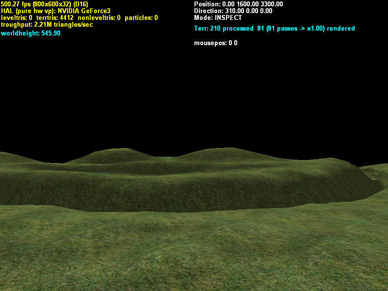
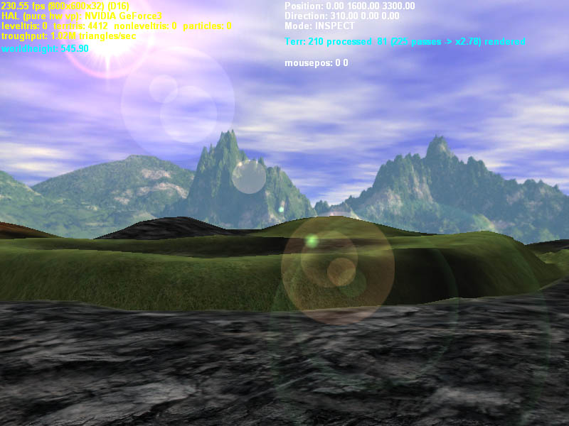
Results
Table 1 shows frame rates achieved on an Athlon-1300 with a standard Geforce3. The minimum scene uses just one material together with a lightmap (2 textures in one render pass - see Figure 10a). The full scene renders the same landscape with three materials plus a clouds shadow layer plus a skybox and a large lens flare (7 textures in 4 render passes for the terrain - see Figure 10b).
| Table1: Frame rates achieved at different scene setups and LOD systems. |
The table shows that geomorphing done using the GPU is as almost fast as doing no geomorphing at all. In the minimum scene the software morphing method falls back tremendously since the CPU and the system bus can not deliver the high frame rates (recall that software morphing needs to send all vertices over the bus each frame) achieved by the other methods. Things change when using the full scene setup. Here the software morphing takes advantage of the fact that the terrain is created and sent to the GPU only once but is used four times per frame for the four render passes and that the skybox and lens flare slow down the frame rate independently. Notice that the software morphing method uses the same approach as for hardware morphing. An implementation fundamentally targeted for software rendering would come off far better.
In this article I've shown how to render a dynamically view-dependently triangulated landscape with geomorphing by taking advantage of today's graphics hardware. Splitting the mesh into smaller parts allowed us to apply the described optimizations which lead to achieved high frame rates. Further work could be done to extend the system to use geometry paging for really large terrains. Other open topics are the implementation of different render paths for several graphics card or using a bump map instead of a lightmap in order to achieve dynamic lighting The new generation of DX9 cards allows the use of up to 16 textures per pass which would enable us to draw seven materials plus a cloud shadow layer in just one pass.
Sample Shots
Click onto images to enlarge.
 |
 |
|
| Figure 10a: Terrain with one material layer | Figure 10b: Same 10a but with three materials (grass, stone, mud) + moving cloud layer + skybox + lens flare | |
 |
 |
|
| Figure 10c: Terrain with overlaid triangle mesh | Figure 10d: Getting close to the ground the highly detailed materials become visible | |
 |
 |
|
| Figure 10e: View from the camera's position | Figure 10f: Same scene as 10e from a different viewpoint with same PVS and culling performed |
References
[Air91] John Airey, "Increasing Update Rates in the Building Walkthrough System with Automatic Model-Space Subdivision and Potentially Visible Set Calculations", PhD thesis, University of North Carolina, Chappel Hill, 1991.
[Boe00] Willem H. de Boer, "Fast Terrain Rendering Using Geometrical MipMapping" E-mersion Project, October 2000 (http://www.connectii.net/emersion)
[Cor01] Corel Bryce by Corel Corporation (http://www.corel.com)
[Duc97] M. Duchaineau, M. Wolinski, D. Sigeti, M. Miller, C. Aldrich, M. Mineev-Weinstein, "ROAMing Terrain: Real-time Optimally Adapting Meshes" (http://www.llnl.gov/graphics/ROAM), IEEE Visualization, Oct. 1997, pp. 81-88
[Eva96] Francine Evans, Steven Skiena, and Amitabh Varshney. Optimizing triangle strips for fast rendering. pages 319-326, 1996. (http://www.cs.sunysb.edu/ evans/stripe.html)
[Hop98] H. Hoppe, "Smooth View-Dependent Level-of-Detail Control and its Application to Terrain Rendering" IEEE Visualization 1998, Oct. 1998, pp. 35-42 (http://www.research.microsoft.com/~hoppe)
[Slay95] Wilbur by Joseph R. Slayton. Latest version can be retrieved at http://www.ridgenet.net/~jslayton/software.html
[Sno01] Greg Snook: "Simplified Terrain Using Interlocking Tiles", Game Programming Gems 2, pp. 377-383, 2001, Charles River Media
[Tel91] Seth J. Teller and Carlo H. Sequin. Visibility preprocessing for interactive walkthroughs. Computer Graphics (Proceedings of SIGGRAPH 91), 25(4):61-69, July 1991.
[Usg86] U.S. Geological Survey (USGS) "Data Users Guide 5 - Digital Elevation Models", 1986, Earth Science Information Center (ESIC), U. S. Geological Survey, 507 National Center, Reston, VA 22092 USA
Discuss this article in the forums
Date this article was posted to GameDev.net: 5/8/2003
(Note that this date does not necessarily correspond to the date the article was written)
See Also:
Hardcore Game Programming
Landscapes and Terrain
© 1999-2011 Gamedev.net. All rights reserved. Terms of Use Privacy Policy
Comments? Questions? Feedback? Click here!