Beat Detection Algorithms
Disclaimer
This document is to be distributed for free and without any modification from its original state. The author declines all responsibility in the damage this document or any of the things you will do with it might do to anyone or to anything. This document and any of its contents is not copyrighted and is free of all rights, you may thus use it, modify it or destroy it without breaking any international law. However according to the author's will, you may not use this document for commercial profit directly, but you may use indirectly its intellectual contents; in which case I would be pleased to receive a mail of notice or even thanks. This is my first tutorial and I am still a student, you must assume that this document is probably not free of small errors and bugs. In the same state of mind, those algorithms are not fully optimised, they are explained for pedagogical purposes and you may find some redundant computations or other voluntary clumsiness. Please be indulgent and self criticise everything you might read. Hopefully, lots of this stuff was taken in sources and books of reference; as for the stuff I did: it has proven some true efficiency in test programs I made and which work as wanted. As said in the introduction: If you have any question or any comment about this text, please send it to the above email address, I'll be happy to answer as soon as possible.
Introduction
Simulating a physical phenomena which obeys to known mathematical equations is, with a number of approximations, always feasable. But what about more abstract concepts, such as feelings, which do not follow any laws? The simplest things we can feel are often the hardest things to capture in a program. Beat detection follows this rule : feeling the beat of a song comes naturally to humans or animals. Indeed it is only a feeling one gets when listening to a melody, a feeling which will make you dance in rhythm or hit a table with your hands on the melody beats. Therefore, how can we teach this beat detection to a machine that can only compute logical operations? In fact there are a number of algorithms which manage to approximate, more or less accurately, this beat detection. We will first study the statistical approach of beat detection on a streaming source and secondly a filtering approach of rhythm extraction on a static song.
This guide assumes the reader has basic signal processing understanding (FFT, convolutions and correlations should sound common) maybe some stuff in statistics will also help (Variance, Average, Principal Components Analysis, will be quoted among others). The point here is not to actually write the code of these algorithms, but more to understand how they work and to be able to adapt or create the appropriate algorithm to a situation. If you have a question or a comment about this text, please send it to the above email address, I'll be happy to answer as soon as possible. Anyway, the aim here is to give more precise ideas on the subject of beat detection to the reader. Enjoy.
I – Statistical streaming beat detection
1 – Simple sound energy
a - A first analysis
The human listening system determines the rhythm of music by detecting a pseudo – periodical succession of beats. The signal which is intercepted by the ear contains a certain energy, this energy is converted into an electrical signal which the brain interprets. Obviously, The more energy the sound transports, the louder the sound will seem. But a sound will be heard as a beat only if his energy is largely superior to the sound's energy history, that is to say if the brain detects a brutal variation in sound energy. Therefore if the ear intercepts a monotonous sound with sometimes big energy peaks it will detect beats, however, if you play a continuous loud sound you will not perceive any beats. Thus, the beats are big variations of sound energy. This first analysis will bring us to our simplest model : Sound energy peaks.
In this model we will detect sound energy variations by computing the average sound energy of the signal and comparing it to the instant sound energy. Lets say we are working in stereo mode with two lists of values : (an) and (bn). (an) contains the list of sound amplitude values captured every Te seconds for the left channel, (bn) the list of sound amplitude values captured every Te seconds for the right channel. So we want to compute the instant energy and the average energy of the signal. The instant energy will in fact be the energy contained in 1024 samples (1024 values of a[n] and b[n]), 1024 samples represent about 5 hundreds of second which is pretty much 'instant'. The average energy should not be computed on the entire song, some songs have both intense passages and more calm parts. The instant energy must be compared to the nearby average energy, for example if a song has an intense ending, the energy contained in this ending shouldn't influence the beat detection at the beginning. We detect a beat only when the energy is superior to a local energy average. Thus we will compute the average energy on say : 44032 samples which is about 1 second, that is to say we will assume that the hearing system only remembers of 1 second of song to detect beat. This 1 second time (44032 samples) is what we could call the human ear energy persistence model; it is a compromise between being to big and taking into account too far away energies, and being too small and becoming to close to the instant energy to make a valuable comparison.
The history buffer where we will keep the last 44032 samples wil contain in fact too lists of samples (B[0]) and (B[1]) corresponding to the left (an) and to the right (bn) channels history.
Simple sound energy algorithm #1:
Every 1024 samples:
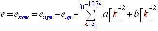
- Use the 1024 new samples taken in a[n] and b[n] to compute the instant energy 'e', using the following formula (i0 is the position of the 1024 samples to process):
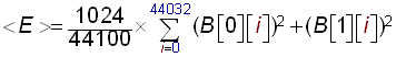
(R1) - Compute the local average energy '<E>' on the 44100 samples of a history buffer (B):
(R2) - Shift the 44032 history buffer (B) of 1024 indexes to the right so that we make room for the 1024 new samples and evacuate the oldest 1024 samples.
- Move the 1024 new samples on top of the history buffer.
- Compare 'e' to 'C * <E>' where C is a constant which will determine the sensibility of the algorithm to beats. A good value for this constant is 1.3. If 'e' is superior to 'C * <E>' then we have a beat!
b - Some direct optimisations
This was the basic version of the algorithm, its speed and accurecy can be improved quite easily. The algorithm can be optimised by keeping the energy values computed on 1024 samples in history instead of the samples themselves, so that we don't have to compute the average energy on the 44100 samples buffer (B) but on the instant energies history we will call (E). This sound energy history buffer (E) must correspond to approximately 1 second of music, that is to say it must contain the energy history of 44032 samples (calculated on groups of 1024) if the sample rate is 44100 samples per second. Thus E[0] will contain the newest energy computed on the newest 1024 samples, and E[42] will contain the oldest energy computed on the oldest 1024 samples. We have 43 energy values in history, each computed on 1024 samples which makes 44032 samples energy history, which is equivalent to 1 second in real time. The count is good. The value of 1 second represents the persistance of the music energy in the human ear, it was obtain with experimentations but it may varry a little from a person to another, just adjust it as you feal. So here is what the algorithm becomes:
Simple sound energy algorithm #2:
Every 1024 samples:
- Compute the instant sound energy 'e' on the 1024 new sample values taken in (an) and (bn) using the formula (R1)
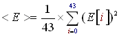
- Compute the average local energy <E> with (E) sound energy history buffer:
(R3) - Shift the sound energy history buffer (E) of 1 index to the right. We make room for the new energy value and flush the oldest.
- Pile in the new energy value 'e' at E[0].
- Compare 'e' to 'C*<E>'.
c - Sensitivity detection
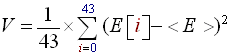
The imediate draw back of this algorithm is the choice of the 'C' constant. For example in techno and rap music beats are quite intense and precise so 'C' should be quite high (about 1.4); whereas for rock and roll, or hard rock which contains a lot of noise, the beats are more confused and 'C' should be low (about 1.1 or 1.0). There is a way, to make the algorithm determine automatically the good choice for the 'C' constant. We must compute the variance of the energies contained in the energy history buffer (E). This variance, which is nothing but the average of ( Energy Values – Energy average = (E) - <E> ), will quantify how marked the beats of the song are and thus will give us a way to compute the value of the 'C' constant. The formula to calculate the variance of the 43 E[i] values is described below (R4). Finally, the greater the variance is the more sensitive the algorithm should be and thus the smaller 'C' will become. We can choose a linear decrease of 'C' with 'V' (the variance) and for example when V → 200, C → 1.0 and when V → 25, C → 1.45 (R5). This is our new version of the sound energy beat detection algorithm:
Simple sound energy algorithm #3:
Every 1024 samples:
- Compute the instant sound energy 'e' on the 1024 new samples taken in (an) and (bn) using the following formula (R1).
- Compute the average local energy <E> with (E) sound energy history buffer using formula (R3).
- Compute the variance 'V' of the energies in (E) using the following formula:
(R4) - Compute the 'C' constant using a linear degression of 'C' with 'V', using a linear regression with values (R5):

(R6) - Shift the sound energy history buffer (E) of 1 index to the right. We make room for the new energy value and flush the oldest.
- Pile in the new energy value 'e' at E[0].
- Compare 'e' to 'C*<E>', if superior we have a beat!
Those three algorithms were tested with several types of music, among others : pop, rock, metal, techno, rap, classical, punk. The fact is the results are quite unpredictable. I will only talk about Simple beat detection algorithm #3 as #2 and #1 are only pedagogical intermediates to get to the #3.
Clearly, the beat detection is very accurate and sounds right with techno and rap, the beats are very precise and the music contains very few noise. The algorithm is quite satisfying for that kind of music and if you aim to use beat detection on techno you can stop reading here, the rest won't change anything to your beat detection. However, even if the improvement of the dynamic 'C' calculations ameliorates things alot, the beat detection on punk, rock and hard rock, is sometimes quite approximate. We can feel it doesn't really get the rythm of the song. Indeed the algorithm detects energy peaks. Sometimes you can hear a drum beat which is sank among other noises and which goes trough the algorithm without being detected as a beat.
To explain this phenomena lets say a guitare and flute make alternatively an amplitude constant note. Each time the first finishes the other starts. The note made by the guitare and the note made by the flute have the same energy but the ear detects a certain rhythm because the notes of the instruments are at different pitch. For our algorithm (who is one might say colorblind) it is just an amplitude constant noise with no energy peaks. This partly explains why the algorithm doesn't detect precisely beats in songs with a lot of instruments playing at different rythms and simultaneously. Our next analysis will make us walk through this difficulty.
Comparing the results we have obtained with the Simple beat detection algorithm #3 to its computing cost, this algorithm is very efficient. If you are not looking for a perfect beat detection than I recommend you use it. Here is a screenshot of a program I made using this algorithm. You fill find the binaries and the sources on my homepage.
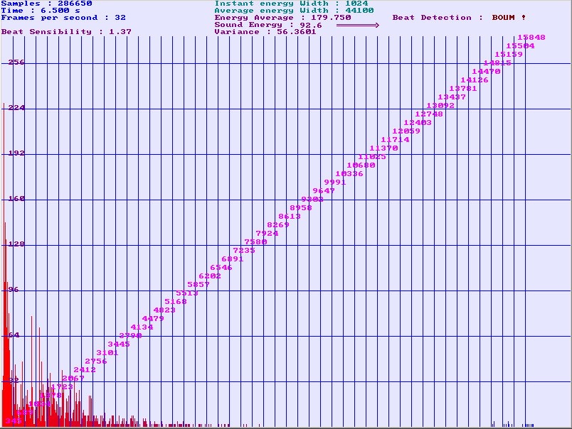
Figure 1: The spectrum analyser is not useful for the beat detection it is only for visual matters, but you can see at the top some of the parameters the program computes to execute the algorithm.
2 – Frequency selected sound energy
a - The idea and the algorithm
The issue with our last analysis of beat detection is that it is colorblind. We have seen that this could raise quite a few problems for noisy like songs in rock or pop music. What we must do is give our algorithm the abbility to determine on which frequency subband we have a beat and if it is powerful enough to take it into account. Basically we will try to detect big sound energy variations in particular frequency subbands, just like in our last analysis; unless this time we will be able to seperate beats regarding their color ( frequency subband ). Thus If we want to give more importants to low frequency beats or to high frequency beats it should be more easy. Notice that the energy computed in the time domain is the same as the energy computed in the frequency domain, so we don't have any difference between computing the energy in time domain or in frequency domain. For maths freaks this is called the Parseval Theorem.
Okay that was just a bit of sport, lets go back to the mainstream; Here is how the Frequency selected sound energy algorithm works: The source signals are still coming from (an) and (bn). (an) and (bn) can be taken from a wave file, or directly from a streaming microphon or line input. Each time we have accumulated 1024 new samples, we will pass to the frequency domain with a Fast Fourier Transform (FFT). We will thus obtain a 1024 frequency spectrum. We then divide this spectrum into however many subbands we like, here I will take 32. The more subbands you have, the more sensitive the algorithm will be but the harder it will become to adapt it to lots of different kinds of songs. Then we compute the sound energy contained in each of the subbands and we compare it to the recent energy average corresponding to this subband. If one or more subbands have an energy superior to their average we have detected a beat.
The great progress with the last algorithm is that we now know more about our beats, and thus we can use this information to change an animation, for example. So here is more precisely the Frequency selected sound energy algorithm #1:
Frequency selected sound energy algorithm #1:
Every 1024 samples:
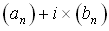
- Compute the FFT on the 1024 new samples taken in (an) and (bn). The FFT inputs a complex numeric signal. We will say (an) is the real part of the signal and (bn) the imagenary part. Thus the FFT will be made on the 1024 complex values of:
You can find FFT tutorials and codes in C, Visual Basic or C++ on my homepage in the 'tutorials' section or by typing 'FFT' on Google.
- From the FFT we obtain 1024 complex numbers. We compute the square of their module and store it into a new 1024 buffer. This buffer (B) contains the 1024 frequency amplitudes of our signal.
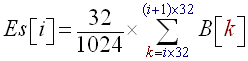
- Divide the buffer into 32 subbands, compute the energy on each of these subbands and store it at (Es). Thus (Es) will be 32 sized and Es[i] will contain the energy of subband 'i':
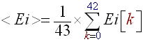
(R7) - Now, to each subband 'i' corresponds an energy history buffer called (Ei). This buffer contains the last 43 energy computations for the 'i' subband. We compute the average energy <Ei> for the 'i' subband simply by using:
(R8) - Shift the sound energy history buffers (Ei) of 1 index to the right. We make room for the new energy value of the subband 'i' and flush the oldest.
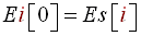
- Pile in the new energy value of subband 'i' : Es[i] at Ei[0].
(R9) - For each subband 'i' if Es[i] > (C*<Ei>) we have a beat !
To help out visualising how the data piles work have a look at this scheme:
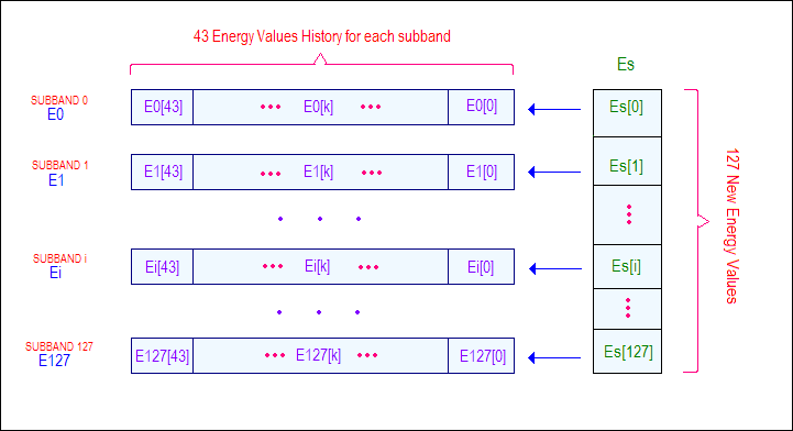
Figure 2: This is how the energy data is organized.
Now the 'C' constant of this algorithm has nothing to do with the 'C' of the first algorithm, because we deal here with separated subbands the energy varies globally much more than with colorblind algorithms. Thus 'C' must be about 250. The results of this algorithm are convincing, it detects for example a symbal rhythm among other heavy noises in metal rock, and indeed the algorithm separates the signal into subbands, therefore the symbal rhythm cannot pass trough the algorithm without being recognized because it is isolated in the frequency domain from other sounds. However the complexity of the algorithm makes it useful only if you are dealing with very noisy sounds, in other cases, Simple beat detection algorithm #3 will do the job.
b - Enhancements and beat decision factors.
There are ways to enhance a bit more our Frequency selected sound energy algorithm #1.
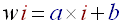
First we will increase the number of subbands from 32 to 64. This will take obviously more computing time but it will also give us more precision in our beat detection. The second way to develop the accuracy of the algorithm uses the defaults of human ears. Human hearing system is not perfect; in fact its transfer function is more like a low pass filter. We hear more easily and more clearly low pitched noises than high pitch noises. This is why it is preferable to make a logarithmic repartition of the subbands. That is to say that subband 0 will contain only say 2 frequencies whereas the last subband, will contain say 20. More precisely the width 'wi' of the 'n' subbands indexed 'i' can be obtained using this argument:
- Linear increase of the width of the subband with its index:
(R10) - We can choose for example the width of the first subband:

(R11) - The sum of all the widths must not exceed 1024 ((B)'s size):
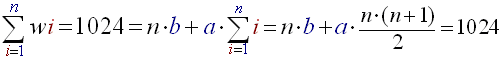
(R12)
Once you have equations (R11) and (R12) it is fairly easy to extract 'a' and 'b', and thus to find the law of the 'wi'. This calculus of 'a' and 'b' must be made manually and 'a' and 'b' defined as constants in the source; indeed they do not vary during the song.
So in fact in Frequency selected sound energy algorithm #1, all we have to modify is the number of subbands we will take equal to 64 and the (R7) relation. This relation becomes:
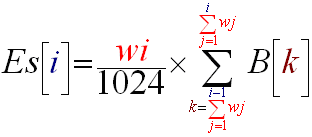
(R7)'
It may seem rather complicated but in fact it is not. Replacing this relation (R7) with (R7)' we have created Frequency selected sound energy algorithm #2. If you have musics with very tight and rapid beats, you may want to compute the stuff more frequently than every 1024 samples, but this is only for special cases, normally the beat should not be shorter than 1/40 of second.
Using the advantages of Frequency selected beat detection you can also enhance the beat decision factor. Up to now it was based on a simple comparison between the instant energy of the subband and the average energy of the subband. This algorithm enables you to decide beats differently. You may want for examples to cut beats which correspond to high pitch sounds if you run techno music or you may want to keep only [50-4000Hz] beats if you are working with speech signal. This algorithm has the advantage of being perfectly adaptable to any kind or category of signal which was not the case of Simple beat detection algorithm #3. Notice that the correspondants between index 'i' of the FFT transform and real frequency is given by formula :
- If 'i' < 'N/2' then:

(R13) - Else 'i' >= 'N/2' then:
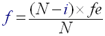
(R14)
So 'i' is the index of the value in the FFT output buffer, N is the size of the FFT transform (here 1024), fe is the sample frequency (here 44100). Thus index 256 corresponds to 10025 Hz. This formula may be useful if you want to create your own subbands and you want to know what the correspondants between indexes and real frequency are.
Another way of filtering the beats, or selecting them, is choosing only those which are marked and precise enough. As we have seen before, to detect the accuracy of beats we must compute the variance of the energy histories for each subband. If this variance is high it means that we have great differences of energy and thus that the beat are very intense. Thus all we have to do is compute this variance for each subband and add a test in the beat detection decision. To the "Es[i] > (C*<Ei>)" condition we will add "and V((Ei))>V0". V0 will be the variance limit, with experience 150 is a reasonable value. Now the V((Ei)) value is easy to compute, just follow the following equality if you don't see how :
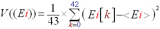
(R15)
The last (finally) way to enhance your beat detection, is to make the source signal pass through a derivation filter. Indeed differentiating the signal makes big variations of amplitude more marked and thus makes energy variations more marked and recognisable later in the algorithm. I haven't tried this optimisation but according to some sources this is quite useful. If you try it please give me your opinion on it!
Concerning the results of the Frequency selected sound energy algorithm #2 I must admit they are way more satisfying than the Simple sound energy algorithm #3. In a song the algorithm catches the bass beats as well as the tight cymbals hits. I insist on the fact that you may also select the beats in very different ways, which becomes quite useful if you know you are going to run techno music with low pitch beats for example. You may also select the beats differently according to there accuracy with the variance criteria. There are many other ways to decide beats; it is up to you to explore them and find the one which fits the most your needs.
I used Frequency selected sound energy algorithm #2algorithm in a demo program of which you can see some screenchots just below. One can see quite clearly that there is a beat in low frequencies (probably a bass or drum hit) and also a high pitch beat (probably a cymbal or such):
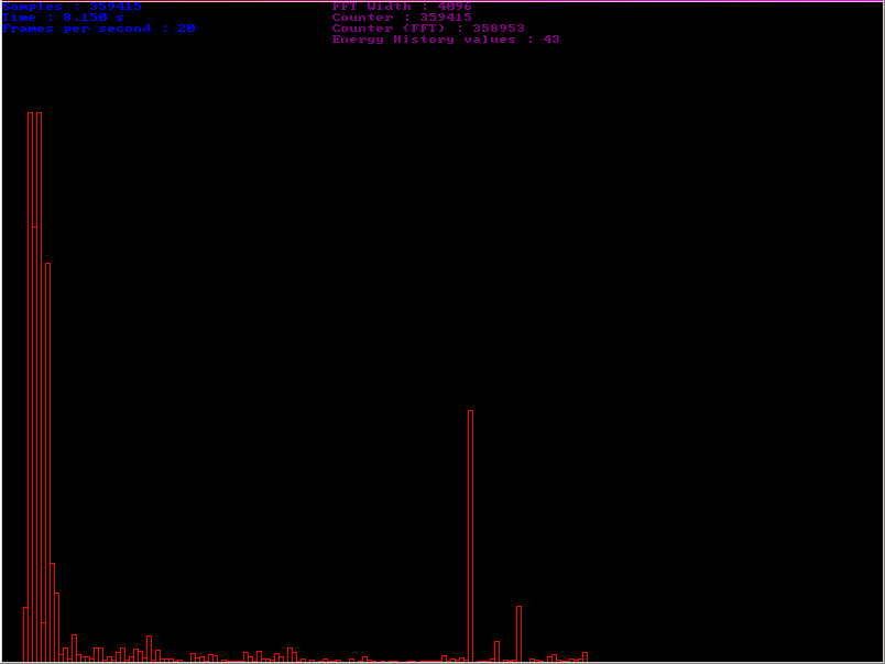
Figure 3: The histogram represents the instant energy of the 128 subbands.
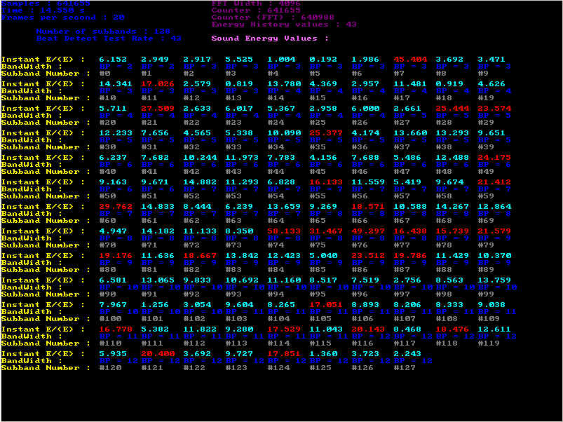
Figure 4: On this screenshot you can see the 128 subbands E/<E> ratios, and the bandwidth of the subbands. When the algorithm detects a beat in a subband, it overwrites the ratio in red.
The reason why I called this part of the document, 'Statistical streaming beat detection', is that the energy can be considered as a random variable, of which we have been calculating values over time. Thus we could interpret those values as a sampling for the statistical analysis of a random variable. But one can push this approach further. When we have separated the energies histories into 128 subbands we created in fact 128 random energy variables. We can then apply some of the general statistical methods of analysis. For example, the principal components analysis method will enable you to determine if some of the subbands are directly linked or independent. This would help us to regroup some subbands which are directly linked and thus make the beat decision more efficient. However, this method is basically just far too computing expensive and maybe just too hard to implement comparing to the results we want. If you are looking for a really good challenge in beat detection you could push in this direction.
II – Filtering rhythm detection
1 – Derivation and Comb filters
a - Intercorrelation and train of impulses
While in the first part of this document we had seen beat detection as a statistical sound energy problem, we will approach it here as a signal processing issue. I haven't tried myself this algorithm but I greatly inspired myself of some work which was done and tested with this algorithm (see the sources section), so it really works but I won't detail so much its implementation as I did in the first part. The basic idea is the following. If we have two signals x(t) and y(t), we can evaluate a function which will give us an idea of how much those two signals are similar. This function called 'inter correlation function' is the following:
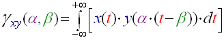
(R16)
For our purposes we will always take alpha=1. This function quantifies the energy that can be exchanged between the signal x(t) and the signal y(t – β), it gives an evaluation of how much those two functions look like each other. The role of the 'β' is to eliminate the time origin problem; two signals should be compared without regarding their possible time axis translation. As you may have noticed, we are creating this algorithm for a computer to execute; basically we have to re-write this formula in discrete mode, it becomes:
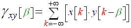
(R17)
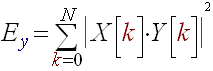
Now the point is we can valuate the similarity of our song and of a train of impulses using this function. The train of impulses being at a known frequency (the beats per minute we want to test) is what we call a comb filter. The energy of the γ function gives us an evaluation of the similarity between our song and this train of impulses, thus it quantifies how much the rhythm of the train of impulses is present in the song. If we compute the energy of the γ function for different train of impulses, we will be able to see for which of them the energy is the biggest, and thus we will know what is the principal Betas Per Minute rate. This is called combfilter processing. We will note 'Ey' this energy, where x[k] is our song signal and y[k] our train of impulses:

(R18)
By the way, here is what a train of impulses looks like:
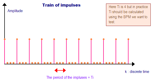
Figure 5: This is the train of impulses function, it is caracterised by its period Ti.
So the period Ti of the impulses must correspond to the beats per minutes we want to test on our song. The formula that links a beat per minute value with the Ti in discrete time is the following:

(R19)
fs is the sample frequency, if you are using good quality wave files, it is usually of 44100. BPM is the beats per minute rate. Finally, Ti is the number of indexes between each impulse.
Now because it is quite computing expensive to compute the (R17) formula, we pass to the frequency domain with a FFT and compute the product of the X[v] and Y[v] (FFT's of x[k] and y[k]). Then we compute the energy of the γ function directly in the frequency domain, thus Ey is given with by the following formula:
(R17)'
b - The algorithm
Note that this algorithm is much too computing expensive to be ran on a streaming source, or on a song in a whole. It is executed on a part of the song, like 5 seconds taken somewhere in the middle. Thus we assume that the tempo of the song is overall constant and that the middle of the song is tempo-representative of the rest of the song. So finally here are the steps of our algorithm:
Derivation and Combfilter algorithm #1:
- Choose roughly 5 seconds of data in the middle of the song and copy it to the 'a[k]' and 'b[k]' lists. The dimension of those lists is noted N. As usual 'a[k]' is the array for the left values, and 'b[k]' is the array for the right values.
- Compute the FFT of the complex signal made with a[k] for the real part of the complex signal and b[k] the imaginary part of the complex signal as seen in Frequency selected sound energy algorithm #1. Store the real part of the result in ta[k] and the imaginary in tb[k].
- For all the beats per minute you want to test, for example from 60 BPM to 180 BPM per step of 10, we will note BPMc the current BPM tested:
- Compute the Ti value corresponding to BPMc using formula (R19).
- Compute the train of impulses signal and store it in (l) and (j). (l) and (j) are purely identical, we take two lists of values to have a stereo signal so that we don't have dimension issues further on. Here is how the train of impulses is generated:
for (k = 0; k < N; k++) { if ((k % Ti) == 0) l[k] = j[k] = AmpMax; else l[k] = j[k] = 0; } - Compute the FFT of the complex signal made of (l) and (j). Store the result in tl[k] and tj[k].
- Finally compute the energy of the correlation between the train of impulses and the 5 seconds signal using (R17)' which becomes:
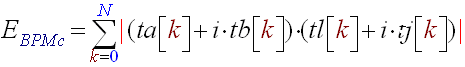
(R20) - Save E(BPMc) in a list.
- The rhythm of the song is given by the BPMmax, where the max of all the E(BPMc) is taken. We have the beat rate of the song!
The AmpMax constant which appears in the train of impulse generation, is given by the sample size of the source file. Usually the sample size is 16 bits, for a good quality .wav. If you are working in non-signed mode, the AmpMax value will be of 65535, and more often if you work with 16 bits signed samples the AmpMax will be 32767.
One of the first ameliorations that could be given to Derivation and Combfilter algorithm #1 is indeed adding a derivation filter before the combfilter processing. To make beats more detectable, we differentiate the signal. This accentuates when the sound amplitude changes. So instead of dealing with a[k] and b[k] directly we first transform them using the formula below. This modification added before the second step of Derivation and Combfilter algorithm #1 constitutes Derivation and Combfilter algorithm #2.
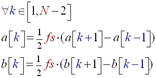
(R21)
As I said before, I haven't tested this algorithm myself; I can't compare its results with the algorithms of the first part. However, throughout the researches I made this seems to be the algorithm universally accepted as being the most accurate. It does have disadvantages: Great computing power consumption, can only be done on a small part of a song, assumes the rhythm is constant throughout the song, no possible streaming input (for example from a microphone), the signal needs to be known in advance. However it returns a deeper analysis than the first part algorithms, indeed for each BPM rate you have a value of its importance in the song.
2 – Frequency selected processing
a - Curing colorblindness
As in the first part of the tutorial, we have the same problem our last algorithm doesn't make the difference between cymbals beat or a drum beat, so the beat detection becomes a bit dodgy on very noisy music like hard rock. To heal our algorithm we will proceed as we had done in Frequency selected sound energy algorithm #1 we will separate our source signal into several subbands. Only this time we have much more computing to do on each subband so we will be much more limited in their number. I think that 16 is a good value. We will use a logarithmic repartition of these subbands as we had done before.
Let's modify the Derivation and Combfilter algorithm #2. The values particular to a subband will be characterized with a little 's' at the end of the name of the variable. So we will separate ta[k] and tb[k] into 16 subbands. Each subbands values array will be called tas[k] and tbs[k] ('s' varies from 1 to 16).
Frequency selected processing combfilters algorithm #1:
- Choose roughly 5 seconds of data in the middle of the song and copy it to the 'a[k]' and 'b[k]' lists. The dimension of those lists is noted N. As usual 'a[k]' is the array for the left values, and 'b[k]' is the array for the right values.
- Differentiate the a[k] and b[k] signals using (R21).
- Compute the FFT of the complex signal made with a[k] for the real part of the complex signal and b[k] the imaginary part of the complex signal as seen in Frequency selected sound energy algorithm #1. Store the real part of the result in ta[k] and the imaginary in tb[k].
- Generate the 16 subband array values tas[k] and tbs[k] by cutting ta[k] and tb[k] with a logarithmic rule.
- For all the subbands tas[k] and tbs[k] (s goes from 1 to 16). Ws is the length of the 's' subband.
- For all the beats per minute you want to test, for example from 60 BPM to 180 BPM per step of 10, we will note BPMc the current BPM tested :
- Compute the Ti value corresponding to BPMc using formula (R19).
- Compute the train of impulses signal and store it in (l) and (j). (l) and (j) are purely identical, we take two lists of values to have a stereo signal so that we don't have dimension issues further on. Here is how the train of impulses is generated:
for (k = 0; k < ws; k++) { if ((k % Ti) == 0) l[k] = k[k] = AmpMax; else l[k] = j[k] = 0; } - Compute the FFT of the complex signal made of (l) and (j). Store the result in tl[k] and tj[k].
- Finally compute the energy of the correlation between the train of impulses and the 5 seconds signal using (R17)' which becomes:

(R22) - Save E(BPMc,s) in a list.
- The rhythm of the subband is given by the BPMmaxs, where the max of all the E(BPMc,s) is taken (s is fixed). We will call this max EBPMmaxs. We have the beat rate of the subband we store it in a list.
- We do this for all the subbands, we have a list of BPMmaxs for all subbands, we can than decide which one to consider.
As in Frequency selected sound energy algorithm #2 we will then be able to decide the rhythm according to frequency bandwidth criteria. Or, if you want to take all the subbands into account you can compute the final BPM of the song, by calculating the barycentre of all the BPMmaxs affected with their max of E(BPMc,s). Like this:
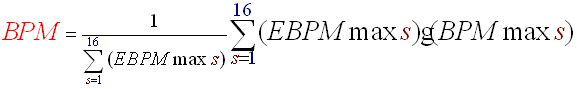
(R23)
I must admit I haven't concretely tested this algorithm. Others have done this already and here an overview of the results for Derivation and Combfilter algorithm #2 (source: http://www.owlnet.rice.edu/~elec301/Projects01/beat_sync/beatalgo.html).
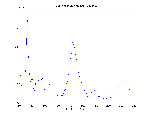
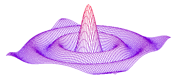
Figure 6: This is plot of the EBPMc values function of BPMc. The algorithm will take the max of the EBPMc value to find the final BPM of the song. Here we see this max is reached for BPMc=75. The final BPM is 75!
Conclusion
Finding algorithms for beat detection is very frustrating. It seems so obvious to us, humans, to hear those beats and somehow so hard to formalise it. We managed to approximate more or less accurately and more or less efficiently this beat detection. But the best algorithms are always the ones you make yourself, the ones which are adapted to your problem. The more the situation is precise and defined the easier it is! This guide should be used as a source of ideas. Even if beat detection is far from being a crucial topic in the programming scene, it has the advantage of using lots of signal processing and mathematical concepts. More than an end in itself, for me, beat detection was a way to train to signal processing. I hope you will find some of this stuff useful.
Sources and Links
- http://www.owlnet.rice.edu/~elec301/Projects01/beat_sync/beatalgo.html : This site greatly inspired me for the second part of the tutorial, very well explained.
- http://www.cs.princeton.edu/~gessl/papers/amta2001.pdf : Audio analysis using the discrete wavelet transform.
- Tempo and beat analysis of acoustic musical signals by Eric D. Scheirer
- Pacemaker by Olli Parviainen
Discuss this article in the forums
Date this article was posted to GameDev.net: 6/7/2003
(Note that this date does not necessarily correspond to the date the article was written)
See Also:
Featured Articles
General
© 1999-2011 Gamedev.net. All rights reserved. Terms of Use Privacy Policy
Comments? Questions? Feedback? Click here!