Disclaimer
This document is to be distributed for free and without any modification from its original contents. The author declines all responsibility in the damage this document or any of the things you will do with it might do to anyone or to anything. This document (and any of its contents) is not copyrighted and is free of all rights, you may thus use it, modify it or destroy it without breaking any international law.
However, there are no warranties or such that the content of the document is error proof. If you found an error please check the latest version of this paper on my homepage before mailing me.
According to the author's will, you may not use this document for commercial profit directly, but you may use indirectly its intellectual contents; in which case I would be pleased to receive a mail of notice or even thanks. The algorithms and methods explained in this article are not totally optimised, they are sometimes simplified for pedagogical purposes and you may find some redundant computations or other voluntary clumsiness. Please be indulgent and self criticise everything you might read. Hopefully, lots of this stuff was taken in sources and books of reference; as for the stuff I did: it has proven some true efficiency in test programs I made and which work as wanted. As said in the introduction: If you have any question or any comment about this text, please send it to the above email address, I'll be happy to answer as soon as possible. Finally, notice that all the source code quoted in this article is available here: http://teachme.free.fr/dsp.zip. You will need the Allegro graphical library and preferably Microsoft Visual C++ 6.0 to compile the project.
Introduction
Digital image processing remains a challenging domain of programming for several reasons. First the issue of digital image processing appeared relatively late in computer history, it had to wait for the arrival of the first graphical operating systems to become a true matter. Secondly, digital image processing requires the most careful optimisations and especially for real time applications. Comparing image processing and audio processing is a good way to fix ideas. Let us consider the necessary memory bandwidth for examining the pixels of a 320x240, 32 bits bitmap, 30 times a second: 10 Mo/sec. Now with the same quality standard, an audio stereo wave real time processing needs 44100 (samples per second) x 2 (bytes per sample per channel) x 2 (channels) = 176Ko/sec, which is 50 times less.
Obviously we will not be able to use the same signal processing techniques in both audio and image. Finally, digital image processing is by definition a two dimensions domain; this somehow complicates things when elaborating digital filters.
We will explore some of the existing methods used to deal with digital images starting by a very basic approach of colour interpretation. As a more advanced level of interpretation comes the matrix convolution and digital filters. Finally, we will have an overview of some applications of image processing.
This guide assumes the reader has a basic signal processing understanding (Convolutions and correlations should sound common places) and also some algorithmic notions (complexity, optimisations). The aim of this document is to give the reader a little overview of the existing techniques in digital image processing. We will neither penetrate deep into theory, nor will we in the coding itself; we will more concentrate on the algorithms themselves, the methods. Anyway, this document should be used as a source of ideas only, and not as a source of code. If you have a question or a comment about this text, please send it to the above email address, I'll be happy to answer as soon as possible. Please enjoy your reading.
I – A simple approach to image processing
1 – The colour data: Vector representation
a - Bitmaps
The original and basic way of representing a digital colored image in a computer's memory is obviously a bitmap. A bitmap is constituted of rows of pixels, contraction of the words 'Picture Element'. Each pixel has a particular value which determines its appearing color. This value is qualified by three numbers giving the decomposition of the color in the three primary colors Red, Green and Blue. Any color visible to human eye can be represented this way. The decomposition of a color in the three primary colors is quantified by a number between 0 and 255. For example, white will be coded as R = 255, G = 255, B = 255; black will be known as (R,G,B) = (0,0,0); and say, bright pink will be : (255,0,255). In other words, an image is an enormous two-dimensional array of color values, pixels, each of them coded on 3 bytes, representing the three primary colors. This allows the image to contain a total of 256x256x256 = 16.8 million different colors. This technique is also know as RGB encoding, and is specifically adapted to human vision. With cameras or other measure instruments we are capable of 'seeing' thousands of other 'colors', in which cases the RGB encoding is inappropriate.
The range of 0-255 was agreed for two good reasons: The first is that the human eye is not sensible enough to make the difference between more than 256 levels of intensity (1/256 = 0.39%) for a color. That is to say, an image presented to a human observer will not be improved by using more than 256 levels of gray (256 shades of gray between black and white). Therefore 256 seems enough quality. The second reason for the value of 255 is obviously that it is convenient for computer storage. Indeed on a byte, which is the computer's memory unit, can be coded up to 256 values.
As opposed to the audio signal which is coded in the time domain, the image signal is coded in a two dimensional spatial domain. The raw image data is much more straight forward and easy to analyse than the temporal domain data of the audio signal. This is why we wiil be able to do lots of stuff and filters for images without tranforming the source data, this would have been totally impossible for audio signal. This first part deals with the simple effects and filters you can compute without transforming the source data, just by analysing the raw image signal as it is.
The standard dimensions, also called resolution, for a bitmap are about 500 rows by 500 columns. This is the resolution encountered in standard analogical television and standard computer applications. You can easily calculate the memory space a bitmap of this size will require. We have 500 x 500 pixels, each coded on three bytes, this makes 750 Ko. It might not seem enormous compared to the standards of hard drives but if you must deal with an image in real time processing things get tougher. Indeed rendering images fluidly demands a minimum of 30 images per second, the required bandwidth of 10 Mo/sec is enormous. We will see later that the limitation of data access and transfer in RAM has a crucial importance in image processing, and sometimes it happens to be much more important than limitation of CPU computing, which may seem quite different from what one can be used to in optimization issues. Notice that, with modern compression techniques such as JPEG 2000, the total size of the image can be easily divided by 50 without losing a lot of quality, but this is another topic.
b – Vector representation of colors
As we have seen, in a bitmap, colors are coded on three bytes representing their decomposition on the three primary colours. It sounds obvious to a mathematician to immediately interpret colors as vectors in a three dimension space where each axis stands for one of the primary colors. Therefore we will benefit of most of the geometric mathematical concepts to deal with our colors, such as norms, scalar product, projection, rotation or distance. This will be really interesting for some kind of filters we will see soon. Figure 1, illustrates this new interpretation:
Figure 1 : Vector representation of colors
2 – Immediate application to filters
a – Edge Detection
From what we have said before we can quantify the 'difference' between two colors by computing the geometric distance between the vectors representing those two colors. Lets consider two colors C1 = (R1,G1,B1) and C2 = (R2,B2,G2), the distance between the two colors is given by the formula :

(R1)
This leads us to our first filter: edge detection. The aim of edge detection is to determine the edge of shapes in a picture and to be able to draw a result bitmap where edges are in white on black background (for example). The idea is very simple; we go through the image pixel by pixel and compare the colour of each pixel to its right neighbour, and to its bottom neighbour. If one of these comparison results in a too big difference the pixel studied is part of an edge and should be turned to white, otherwise it is kept in black. The fact that we compare each pixel with its bottom and right neighbour comes from the fact that images are in two dimensions. Indeed if you imagine an image with only alternative horizontal stripes of red and blue, the algorithms wouldn't see the edges of those stripes if it only compared a pixel to its right neighbour. Thus the two comparisons for each pixel are necessary. So here is the algorithm in symbolic language and in C.
Algorithm 1 : Edge Detection
- For every pixel ( i , j ) on the source bitmap
- Extract the (R,G ,B) components of this pixel, its right neighbour (R1,G1,B1), and its bottom neighbour (R2,G2,B2)
- Compute D(C,C1) and D(C,C2) using (R1)
- If D(C,C1) OR D(C,C2) superior to a parameter K, then we have an edge pixel !
Translated in C language using allegro 4.0 (references in the sources) gives:
for(i=0;i<temp->w-1;i++){
  for(j=0;j<temp->h-1;j++){

    color=getpixel(temp,i,j);
    r=getr32(color);
    g=getg32(color);
    b=getb32(color);

    color1=getpixel(temp,i+1,j);
    r1=getr32(color1);
    g1=getg32(color1);
    b1=getb32(color1);

    color2=getpixel(temp,i,j+1);
    r2=getr32(color2);
    g2=getg32(color2);
    b2=getb32(color2);

    if((sqrt((r-r1)*(r-r1)+(g-g1)*(g-g1)+(b-b1)*(b-b1))>=bb)||
       (sqrt((r-r2)*(r-r2)+(g-g2)*(g-g2)+(b-b2)*(b-b2))>=bb)){

      putpixel(temp1,i,j,makecol(255,255,255));

    }
    else{
      putpixel(temp1,i,j,makecol(0,0,0));
    }
  }
}
This algorithm was tested on several source images of different types and it gives fairly good results. It is mainly limited in speed because of frequent memory access. The two square roots can be removed easily by squaring the comparison; however, the colour extractions cannot be improved very easily. If we consider that the longest operations are the getpixel function,get*32 and putpixel functions, we obtain a polynomial complexity of 4*N*M, where N is the number of rows and M the number of columns. This is not reasonably fast enough to be computed in real time. For a 300x300x32 image I get about 26 transforms per second on an Athlon XP 1600+. Quite slow indeed.
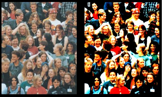
Here are the results of the algorithm on an example image:
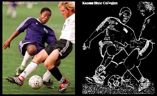
Picture 1 : Edge detection Results
A few words about the results of this algorithm: Notice that the quality of the results depends on the sharpness of the source image. If the source image is very sharp edged, the result will reach perfection. However if you have a very blurry source you might want to make it pass through a sharpness filter first, which we will study later. Another remark, you can also compare each pixel with its second or third nearest neighbours on the right and on the bottom instead of the nearest neighbours. The edges will be thicker but also more exact depending on the source image's sharpness. Finally we will see later on that there is another way to make edge detection with matrix convolution.
b – Color extraction
The other immediate application of pixel comparison is color extraction. Instead of comparing each pixel with its neighbors, we are going to compare it with a given color C1. This algorithm will try to detect all the objects in the image that are colored with C1. This was quite useful for robotics for example. It enables you to search on streaming images for a particular color. You can then make you robot go get a red ball for example. We will call the reference color, the one we are looking for in the image C0 = (R0,G0,B0).
Algorithm 2 : Color extraction
- For every pixel ( i , j ) on the source bitmap
- Extract the C = (R,G ,B) components of this pixel.
- Compute D(C,C0) using (R1)
- If D(C,C0) inferior to a parameter K, we found a pixel which colour's matches the colour we are looking for. We mark it in white. Otherwise we leave it in black on the output bitmap.
Translated in C language using Allegro 4.0 (references in the sources) gives:
for(i=0;i<temp->w-1;i++){
  for(j=0;j<temp->h-1;j++){

    color=getpixel(temp,i,j);
    r=getr32(color);
    g=getg32(color);
    b=getb32(color);

    if(sqrt((r-r0)*(r-r0)+(g-g0)*(g-g0)+(b-b0)*(b-b0))<=aa){

      putpixel(temp1,i,j,makecol(255,255,255));
    }
    else{

      putpixel(temp1,i,j,makecol(0,0,0));
    }
  }
}
Once again, even if the square root can be easily removed it doesn't really affect the speed of the algorithm. What really slows down the whole loop is the NxM getpixel accesses to memory and the get*32 and putpixel. This determines the complexity of this algorithm: 2xNxM, where N and M are respectively the numbers of rows and columns in the bitmap. The effective speed measured on my computer is about 40 transforms per second on a 300x300x32 source bitmap. Here are the results I obtained using this algorithm searching for whites shape in the source bitmap:
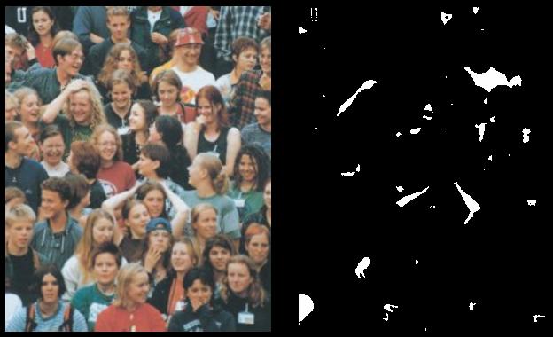
Picture 2 : White Extraction Results
c – Color to grayscale conversion
Regarding the 3D color space, grayscale is symbolized by the straight generated by the (1,1,1) vector. Indeed, the shades of grays have equal components in red, green and blue, thus their decomposition must be (n,n,n), where n is an integer between 0 and 255 (example : (0,0,0) black, (32,32,32) dark gray, (128,128,128) intermediate gray, (192,192,192) bright gray, (255,255,255) white etc…). Now the idea of the algorithm is to find the importance a color has in the direction of the (1,1,1) vector. We will use scalar projection to achieve this. The projection of a color vector C = (R,G,B) on the vector (1,1,1) is computed this way :

(R2)

(R3)
However the projection value can reach up to 441.67, which is the norm of the white color (255,255,255). To avoid having numbers above 255 limit we will multiply our projection value by a factor 255/441,67=1/sqrt(3). Thus the formula simplifies a little giving:

(R4)
So in fact converting a color to a grayscale value is just like taking the average of its red, green and blue components. You can also adapt the (R3) formula to other color-scales. For example you can choose to have a red-scale image, Redscale(C)=R, or a yellow-scale image, Yellowscale(C)=(G+B)/sqrt(6) etc…
Algorithm 3 : Grayscale conversion
- For every pixel ( i , j ) on the source bitmap
- Extract the C = (R,G ,B) components of this pixel.
- Compute Grayscale(C) using (R4)
- Mark pixel ( i , j ) on the output bitmap with color (Grayscale(C), Grayscale(C), Grayscale(C)).
C source code equivalent is :
for(i=0;i<temp->w-1;i++){
  for(j=0;j<temp->h-1;j++){

    color=getpixel(temp,i,j);
    r=getr32(color);
    g=getg32(color);
    b=getb32(color);

    h=(r+b+g)/3;
    putpixel(temp1,i,j,makecol(h,h,h));
  }
}
It's impossible to optimize this algorithm regarding its simplicity but we can still give its computing complexity which is given by the number of pixel studied: NxM, (N,M) is the resolution of the bitmap. The execution time on my computer is the same as in the previous algorithm, still about 35 transforms per second. Here is the result of the algorithm on a picture:
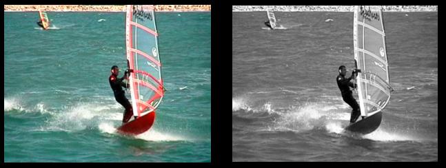
Picture 3 : Grayscale conversion Results
3 – Grayscale transforms: light and contrast
a – Grayscale transforms
Grayscale transforms are integer functions from [0,255] to [0,255], thus to any integer value between 0 and 255 we make another value between 0 and 255 correspond. To obtain the image of a color by a grayscale transform, it must be applied to the three red, green and blue components separately and then reconstitute the final color. The graph of grayscale transform is called an output look-up table, or gamma-curve. In practice you can control the gamma-curve of your video-card to set lightness or contrast, so that each time it sends a pixel to the screen, it makes it pass through the grayscale transform first. Here are the effects of increasing contrast and lightness to the gamma-curve of the corresponding grayscale transform:
 |
 |
| Normal grayscale transform |
Increased brightness by 128 |
 |
 |
| Decreased brightness by 128 |
Increased contrast by 15° |
 |
 |
| Increased contrast by 30° |
Increased contrast by 30° at 64 and 150 |
 |
|
| Increased brightness and contrast |
Figure 2 : Basic grayscale transforms
Notice that if you want to compose brightness and contrast transforms you should first apply the contrast transform and then the brightness transform. One can also easily create his own grayscale transform to improve the visibility of an image. For example, if you have a very dark image with a small bright zone in it. You cannot increase a lot brightness because the bright zone will saturate quickly but the idea is to increase the contrast exactly where there are the most pixels, in this case: for low values of colors (dark). This will have the effect of flattening the colors histogram and making the image use a wider range of colors, thus making it more visible. So, first the density histogram must be built, counting the number of pixels for each 0-255 value. Then we built the contrast curve we want, finally we integrate to obtain the final transform. The integration comes from the fact that contrast is a slope value, therefore to come back to the contrast transform function we must integrate. Those figures explain this technique:
 |
 |
| Bitmap input color histogram: two large amounts of pixels in thin color bandwidths. |
The contrast slope must be big in those two areas to flatten the input histogram. |
 |
 |
| The contrast transform: It is obtained by integrating the previous plot. |
The input bitmap color histogram before and after the contrast transform: Now pixels are averagely distributed on the whole color bandwidth. |
Figure 3 : Custom grayscale transforms
b – Light and contrast
Light and contrast transforms are immediate to implement: once the output look-up table is saved into memory once and for all, each pixel is passed trough this table and marked on the output bitmap. The look-up table will be represented simply as a list. The index of the list will stand for the input color value and the contents of the list will be the output. So calling list[153] will give us the image of grayscale level 153 by our transform.
Algorithm 4 : Light or contrast modification
- Generate the look-up table for the desired transform (Light or contrast or any other). For each index j from 0 to 255 is stored its image by the transform in transform_list[ j ].
- For every pixel ( i , j ) on the source bitmap
- Extract the C = (R,G ,B) components of this pixel.
- Mark pixel ( i , j ) on the output bitmap with color (transform_list[R], transform_list[G], transform_list[B]).
In the C source code implementation for contrast, the float variable contrast quantifies the angle of the slope (in radians) of the contrast transform like in figure 2. If contrast is defined as pi/4 there will be no changes in the image, as this corresponds to the 'normal' transform of figure 2. Significant changes start when contrast > pi/4 + 15°. If contrast reaches 0 all the image will be gray because the transform will be a horizontal straight at 128. If contrast becomes very big, any color value becomes either 0 or 255 depending on its position around 128, so the output bitmap will have only the 8 possible colors only made of 255 or 0: (255,255,255), (255,255,0), (255,0,255), (0,255,255), (255,0,0), (0,255,0), (0,0,255), (0,0,0).
for(i=0;i<256;i++){
  if(i<(int)(128.0f+128.0f*tan(contrast))&&i>(int)(128.0f-128.0f*tan(contrast)))
    Contrast_transform[i]=(i-128)/tan(contrast)+128;
  else if(i>=(int)(128.0f+128.0f*tan(contrast)))
    Contrast_transform[i]=255;
  else
    Contrast_transform[i]=0;
}

for(i=0;i<temp->w-1;i++){
  for(j=0;j<temp->h-1;j++){

    color=getpixel(temp,i,j);
    r=getr32(color);
    g=getg32(color);
    b=getb32(color);

    putpixel(temp1,i,j,makecol(Contrast_transform[r],Contrast_transform[g],
                               Contrast_transform[b]));
  }
}
C source code implementation for brightness:
for(i=0;i<256;i++){
  Light_transform[i]=i+light;
  if(Light_transform[i]>255)
    Light_transform[i]=255;
  if(Light_transform[i]<0)
    Light_transform[i]=0;
}

for(i=0;i<temp->w-1;i++){
  for(j=0;j<temp->h-1;j++){

    color=getpixel(temp,i,j);
    r=getr32(color);
    g=getg32(color);
    b=getb32(color);

    putpixel(temp1,i,j,makecol(Contrast_transform[r],Contrast_transform[g],
                               Contrast_transform[b]));
  }
}
The efficiency of the algorithm is limited by the getpixel and putpixel calls and the speed is the same as the last two algorithms: about 40 transforms per second on my computer. Here are some examples of outputs:
Picture 4 : Brightness transform result
Picture 5 : Contrast transform result
4 – Resizing and rotating algorithms
a – Resizing algorithm
The resizing of an image is far from being trivial. A few techniques exist, each giving more or less good results in stretching or squeezing. Linear resizing is what we will be studying here, I haven't experienced other methods and I won't be able to compare linear resizing with other methods. However, the resizing process is rarely something done for real-time matters. The aim is usually to resize the image once, and if the algorithm takes 5 seconds or 10 ms, it doesn't matter much. For this kind of algorithm quality is put ahead of speed. For the following explanation let E(x) be the integer part of x (E(3.14) = 3) and F(x) the fractional part of x (E(3.14) = 0.14).
We will first see how to stretch or squeeze an image along its width; the process is the same for height and you can cumulate both of them to give the bitmap the desired resolution. Let us consider a row of pixels of the output bitmap of width 'wout'. Let us take a pixel of this row and name his column number xi. To find which color this pixel should be, we are going to convert his column xi to its equivalent column 'ci' in the source bitmap (width = 'win') using the formula:


(R5)
Thus pixel in column 'xi' in the output bitmap should be in fact the same color as pixel in column 'ci' in the source bitmap. The problem is that 'ci' is a floating point value and one cannot access floating point pixel numbers (no surprise). However, 'ci' falls in between two integer column numbers E(ci) and E(ci)+1 which can be accessed. You can simply convert 'ci' to its actual integer value: E(ci) and choose the color at pixel E(ci) in the source image. This constitutes the 'nearest neighbour' method. There is another way to solve the problem that has the advantage of giving nicer results at high enlarging ratios: linear interpolation.
In fact, the final color we will choose for pixel 'xi' is not exactly that of pixel 'E(ci)' but a linear interpolation between the color of 'E(ci)' and 'E(ci)'+1 using the fractional part of 'ci'. Thus the final color we will choose for the color of the 'xi' pixel in the output bitmap will be computed by this formula:

(R6)
Therefore, when stretching the image, the algorithm will try to compensate the lack of information due to the increase of pixels by using linear interpolation. The difference between choosing linear interpolation to compute the color or simply pick the color at 'E(ci)' is not flabbergasting, but the second gives a nice smooth effect and when you have enormous stretches ratio it looks quite nicer than the first one. The first method is more commonly called 'nearest neighbour' and second one is know as 'bi-linear'. Photoshop© uses a third method called 'bi-cubic', but I don't know about it. I used linear interpolation for this screenshot:
Picture 6 : Resizing algorithm result
Figure 4: Color interpolation in stretching image
The code in C and the algorithm implementing this resizing methods:
Algorithm 5 : Resizing a bitmap
- First we resize the width of the bitmap:
- For every pixel ( i , j ) on the output bitmap
- Compute the ci using formula (R5)
- Extract the (R,G,B) components of pixel E(ci) and E(ci)+1 in source bitmap using (R6)
- Mark pixel ( i , j ) on the output bitmap with color given by formula (R7)
- Repeat the exact same process to resize the height of the bitmap
bs=(float)temp->w/(float)size;

for(i=1;i<size;i++){
  for(j=1;j<temp->h-1;j++){

    as=(float)i*bs;
    es=(int)as;
    fs=(int)as+1;

    color=getpixel(temp,es,j);
    r=getr32(color);
    g=getg32(color);
    b=getb32(color);

    colort=getpixel(temp,fs,j);
    rt=getr32(color);
    gt=getg32(color);
    bt=getb32(color);

    cs=modf(as,&gs);

    dr=(float)(rt-r);
    dg=(float)(gt-g);
    db=(float)(bt-b);


    putpixel(temp_size,i,j,makecol((int)(r+(float)cs*dr),
             (int)(g+(float)cs*dg),(int)(b+(float)cs*db)));
    //OR the simple E(ci) method (in which case you can remove lots of stuff above):
    //putpixel(temp_size,i,j,makecol((int)r,(int)g,(int)b));
  }
}
b – Rotation algorithm
Once again there are different ways of implementing bitmap rotation, the faster they are the more complex they get. We will first study a very basic way and then a much more efficient method. As always there is a little bit of mathematics to understand first. Say x and y are the coordinates of a pixel on the bitmap we can find its image (x',y') by the rotation of center (x0,y0) and of angle α by the following formula:
(R8)
If we apply this formula directly, taking each pixel of the source image and passing them through those equations we will obtain lots of holes in the output bitmap. Those wholes are due to the fact that x and y are integers. Necessarily, there will be some x' and y' that will never be reached and which will stay black. The trick is to start from the output image pixels and compute there inverse rotation to find their antecedent by the rotation. Therefore we will use this formula to find (x,y) for every (x',y') of the output bitmap:
(R9)
Once the antecedent pixel is found, we set the output pixel at the same color. Here is the algorithm and the C source:
Algorithm 6 : Rotating a bitmap
- For every pixel (i,j)=(x',y') on the output bitmap
- Compute the antecedent pixel (x,y) of the input image using (R9)
- Mark pixel (i,j) on the output bitmap with the same color as pixel (x,y) of the input bitmap.
cos_val=cos(rangle);
sin_val=sin(rangle);
half_w=temp->w>>1;
half_h=temp->h>>1;

for(j=0;j<temp->h;j++){
  for(i=0;i<temp->w;i++){

    bs=i-half_w;
    cs=j-half_h;

    as=bs*sin_val+cs*cos_val+half_w;
    gs=bs*cos_val-cs*sin_val+half_h;
    color=getpixel(temp,as,gs);
    putpixel(temp1,i,j,color);
  }
}
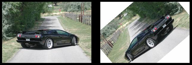
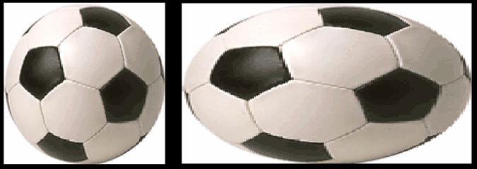
Picture 7 : Rotation algorithm result
With this algorithm I have an even better speed than any of the precedent algorithms, about 42 frames per second. The complexity of the algorithm is N*M where N and M are the dimensions of the source bitmap.
There is a way to improve this algorithm. Instead of computing for each pixel of the output bitmap its inverse rotation, we are going to deal with lines. For each horizontal line in the output image, we compute, as we did before, the inverse rotation of its extreme points. Thus we know the color of all the points of this horizontal line because we know all the color of the pixels on the inverse rotation line on the source bitmap. This way we replace lots of rotations calculations (the ones we did for each pixel on the bitmap) by simple linear interpolation with no multiplications. The difference is not that visible on my machine, I gained 3 fps with this algorithm; moreover, if we look at the complexity, it hasn't change. Indeed even with this linear interpolation there is still N*M pixel accesses. It is really the fact that we avoided all the multiplication of the rotations that makes us win 3 fps.
Algorithm 6 (bis) : Rotating a bitmap
- For every horizontal line in the output bitmap
- Compute the antecedent pixels (x1,y1) and (x2,y2) of the extreme points of the line. (R9)
- For every pixel of line (x1,y1),(x2,y2) on the source image we get its color and set the corresponding pixel on the horizontal line of the output bitmap
cos_val=cos(rangle);
sin_val=sin(rangle);
half_w=temp->w>>1;
half_h=temp->h>>1;

for(j=-1;j<temp->h;j++){
  line_count=0;
  n=j;

  bs=-half_w;
  cs=j-half_h;

  as=bs*cos_val-cs*sin_val+(half_w);
  gs=bs*sin_val+cs*cos_val+(half_h);

  r=as;
  g=gs;

  bs=temp->w-half_w;
  cs=j-half_h;

  as=bs*cos_val-cs*sin_val+(half_w);
  gs=bs*sin_val+cs*cos_val+(half_h);

  do_line(temp1,r,g,(int)as,(int)gs,color,Line_make);

  if(j==-1)
    line_save=line_count;
}

void Line_make(BITMAP* image,int x,int y,int d){

  static int lastx=0;
  int current_color;

  line_count++;

  current_color=getpixel(temp,x,y);

  if(line_count*temp->w/line_save-lastx>1){
    putpixel(temp1,lastx+1,n,current_color);
    putpixel(temp1,lastx+2,n,current_color);
  }
  else{
    putpixel(temp1,line_count*
      temp->w/line_save,n,current_color);
  }
  lastx=line_count*temp->w/line_save;
}
4 – Blending
a – Averages
Blending simply consists in averaging the value of two pixels to get a transparency effect, a mix between the two colors. The average can be more or less equilibrated which gives more or less importance to the first or the second pixel. For example if you want to make a blending between two colors C1 and C2 you can use this formula:

(R10)
Blending is usually done to give transparency effects in 3D games or demos, or transition effects in movies. The blending is often done between two bitmaps, or a bitmap and a color. You can also blend a bitmap with itself, but this results in a sort of blurring which you can achieve much more rapidly with algorithms we will see in the second part of this article. Therefore we will consider we have two bitmaps B1 and B2 we want to blend. They are probably not perfectly edged aligned, and not of the same size. To limit iterations, we copy the biggest bitmap (say B1) on the output bitmap, then we take the smallest bitmap (B2) pixel by pixel, test if the pixel belongs to the other image (B1) at the same time, if it does we average with formula (R10) and set the output pixel, if it doesn't we just set the output pixel directly without changing the color. Anyways once you know that the act of blending is just an averaging, the rest depends on what you want to do.
b – Other blending effects
Blending gives lots of possibilities for cool effects, you can make gradient blending by making the 'α' or 'β' vary; you can have lighting effects, glow effects, transparency effects, water effects, wind effects, lots of the coolest filters in Photoshop© use a simple blending. Once you know this it's rather creativity then technique which makes the difference.
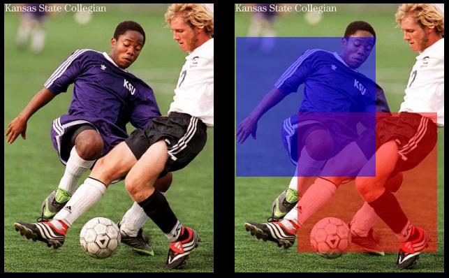
Picture 8 : Blending example

Matrix convolution filters
|
|