II – Filtering rhythm detection
1 – Derivation and Comb filters
a - Intercorrelation and train of impulses
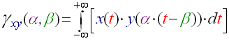
While in the first part of this document we had seen beat detection as a statistical sound energy problem, we will approach it here as a signal processing issue. I haven't tried myself this algorithm but I greatly inspired myself of some work which was done and tested with this algorithm (see the sources section), so it really works but I won't detail so much its implementation as I did in the first part. The basic idea is the following. If we have two signals x(t) and y(t), we can evaluate a function which will give us an idea of how much those two signals are similar. This function called 'inter correlation function' is the following:
(R16)
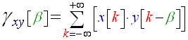
For our purposes we will always take alpha=1. This function quantifies the energy that can be exchanged between the signal x(t) and the signal y(t – β), it gives an evaluation of how much those two functions look like each other. The role of the 'β' is to eliminate the time origin problem; two signals should be compared without regarding their possible time axis translation. As you may have noticed, we are creating this algorithm for a computer to execute; basically we have to re-write this formula in discrete mode, it becomes:
(R17)
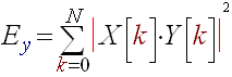
Now the point is we can valuate the similarity of our song and of a train of impulses using this function. The train of impulses being at a known frequency (the beats per minute we want to test) is what we call a comb filter. The energy of the γ function gives us an evaluation of the similarity between our song and this train of impulses, thus it quantifies how much the rhythm of the train of impulses is present in the song. If we compute the energy of the γ function for different train of impulses, we will be able to see for which of them the energy is the biggest, and thus we will know what is the principal Betas Per Minute rate. This is called combfilter processing. We will note 'Ey' this energy, where x[k] is our song signal and y[k] our train of impulses:

(R18)
By the way, here is what a train of impulses looks like:
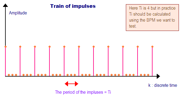
Figure 5: This is the train of impulses function, it is caracterised by its period Ti.
So the period Ti of the impulses must correspond to the beats per minutes we want to test on our song. The formula that links a beat per minute value with the Ti in discrete time is the following:

(R19)
fs is the sample frequency, if you are using good quality wave files, it is usually of 44100. BPM is the beats per minute rate. Finally, Ti is the number of indexes between each impulse.
Now because it is quite computing expensive to compute the (R17) formula, we pass to the frequency
domain with a FFT and compute the product of the X[v] and Y[v] (FFT's of
x[k] and y[k]). Then we compute the energy of the γ function directly in
the frequency domain, thus Ey is given with by the following formula:
(R17)'
b - The algorithm
Note that this algorithm is much too computing expensive to be ran on a streaming source, or on a song in a whole. It is executed on a part of the song, like 5 seconds taken somewhere in the middle. Thus we assume that the tempo of the song is overall constant and that the middle of the song is tempo-representative of the rest of the song. So finally here are the steps of our algorithm:
Derivation and Combfilter algorithm #1:
- Choose roughly 5 seconds of data in the middle of the song and copy it to the 'a[k]' and 'b[k]' lists. The dimension of those lists is noted N. As usual 'a[k]' is the array for the left values, and 'b[k]' is the array for the right values.
- Compute the FFT of the complex signal made with a[k] for the real part of the complex signal and b[k] the imaginary part of the complex signal as seen in Frequency selected sound energy algorithm #1. Store the real part of the result in ta[k] and the imaginary in tb[k].
- For all the beats per minute you want to test, for example from 60 BPM to 180 BPM per step of 10, we will note BPMc the current BPM tested:
- Compute the Ti value corresponding to BPMc using formula (R19).
- Compute the train of impulses signal and store it in (l) and (j). (l) and (j) are purely identical, we take two lists of values to have a stereo signal so that we don't have dimension issues further on. Here is how the train of impulses is generated:
for (k = 0; k < N; k++)
{
  if ((k % Ti) == 0)
    l[k] = j[k] = AmpMax;
  else
    l[k] = j[k] = 0;
}
- Compute the FFT of the complex signal made of (l) and (j). Store the result in tl[k] and tj[k].
- Finally compute the energy of the correlation between the train of impulses and the 5 seconds signal using (R17)' which becomes:
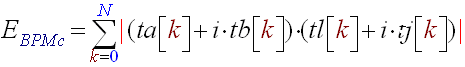
(R20)
- Save E(BPMc) in a list.
- The rhythm of the song is given by the BPMmax, where the max of all the E(BPMc) is taken. We have the beat rate of the song!
The AmpMax constant which appears in the train of impulse generation, is given by the sample size of the source file. Usually the sample size is 16 bits, for a good quality .wav. If you are working in non-signed mode, the AmpMax value will be of 65535, and more often if you work with 16 bits signed samples the AmpMax will be 32767.
One of the first ameliorations that could be given to Derivation and Combfilter algorithm #1 is indeed adding a derivation filter before the combfilter processing. To make beats more detectable, we differentiate the signal. This accentuates when the sound amplitude changes. So instead of dealing with a[k] and b[k] directly we first transform them using the formula below. This modification added before the second step of Derivation and Combfilter algorithm #1 constitutes Derivation and Combfilter algorithm #2.
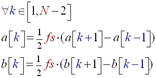
(R21)
As I said before, I haven't tested this algorithm myself; I can't compare its results with the algorithms of the first part. However, throughout the researches I made this seems to be the algorithm universally accepted as being the most accurate. It does have disadvantages: Great computing power consumption, can only be done on a small part of a song, assumes the rhythm is constant throughout the song, no possible streaming input (for example from a microphone), the signal needs to be known in advance. However it returns a deeper analysis than the first part algorithms, indeed for each BPM rate you have a value of its importance in the song.
2 – Frequency selected processing
a - Curing colorblindness
As in the first part of the tutorial, we have the same problem our last algorithm doesn't make the difference between cymbals beat or a drum beat, so the beat detection becomes a bit dodgy on very noisy music like hard rock. To heal our algorithm we will proceed as we had done in Frequency selected sound energy algorithm #1 we will separate our source signal into several subbands. Only this time we have much more computing to do on each subband so we will be much more limited in their number. I think that 16 is a good value. We will use a logarithmic repartition of these subbands as we had done before.
Let's modify the Derivation and Combfilter algorithm #2. The values particular to a subband will be characterized with a little 's' at the end of the name of the variable. So we will separate ta[k] and tb[k] into 16 subbands. Each subbands values array will be called tas[k] and tbs[k] ('s' varies from 1 to 16).
Frequency selected processing combfilters algorithm #1:
- Choose roughly 5 seconds of data in the middle of the song and copy it to the 'a[k]' and 'b[k]' lists. The dimension of those lists is noted N. As usual 'a[k]' is the array for the left values, and 'b[k]' is the array for the right values.
- Differentiate the a[k] and b[k] signals using (R21).
- Compute the FFT of the complex signal made with a[k] for the real part of the complex signal and b[k] the imaginary part of the complex signal as seen in Frequency selected sound energy algorithm #1. Store the real part of the result in ta[k] and the imaginary in tb[k].
- Generate the 16 subband array values tas[k] and tbs[k] by cutting ta[k] and tb[k] with a logarithmic rule.
- For all the subbands tas[k] and tbs[k] (s goes from 1 to 16). Ws is the length of the 's' subband.
- For all the beats per minute you want to test, for example from 60 BPM to 180 BPM per step of 10, we will note BPMc the current BPM tested :
- Compute the Ti value corresponding to BPMc using formula (R19).
- Compute the train of impulses signal and store it in (l) and (j). (l) and (j) are purely identical, we take two lists of values to have a stereo signal so that we don't have dimension issues further on. Here is how the train of impulses is generated:
for (k = 0; k < ws; k++)
{
  if ((k % Ti) == 0)
    l[k] = k[k] = AmpMax;
  else
    l[k] = j[k] = 0;
}
- Compute the FFT of the complex signal made of (l) and (j). Store the result in tl[k] and tj[k].
- Finally compute the energy of the correlation between the train of impulses and the 5 seconds signal using (R17)' which becomes:

(R22)
- Save E(BPMc,s) in a list.
- The rhythm of the subband is given by the BPMmaxs, where the max of all the E(BPMc,s) is taken (s is fixed). We will call this max EBPMmaxs. We have the beat rate of the subband we store it in a list.
- We do this for all the subbands, we have a list of BPMmaxs for all subbands, we can than decide which one to consider.
As in Frequency selected sound energy algorithm #2 we will then be able to decide the rhythm according to frequency bandwidth criteria. Or, if you want to take all the subbands into account you can compute the final BPM of the song, by calculating the barycentre of all the BPMmaxs affected with their max of E(BPMc,s). Like this:
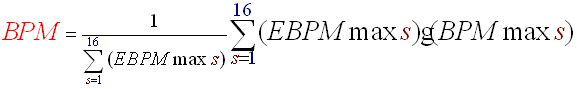
(R23)
I must admit I haven't concretely tested this algorithm. Others have done this already and here an overview of the results for Derivation and Combfilter algorithm #2 (source: http://www.owlnet.rice.edu/~elec301/Projects01/beat_sync/beatalgo.html).
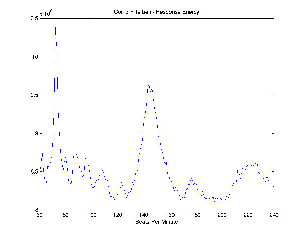
Figure 6: This is plot of the EBPMc values function of BPMc. The algorithm will take the max of the EBPMc value to find the final BPM of the song. Here we see this max is reached for BPMc=75. The final BPM is 75!
Conclusion
Finding algorithms for beat detection is very frustrating. It seems so obvious to us, humans, to hear those beats and somehow so hard to formalise it. We managed to approximate more or less accurately and more or less efficiently this beat detection. But the best algorithms are always the ones you make yourself, the ones which are adapted to your problem. The more the situation is precise and defined the easier it is! This guide should be used as a source of ideas. Even if beat detection is far from being a crucial topic in the programming scene, it has the advantage of using lots of signal processing and mathematical concepts. More than an end in itself, for me, beat detection was a way to train to signal processing. I hope you will find some of this stuff useful.
Sources and Links
|
