Contents  Introduction  Convolution  Code  Filters  Edge Enhancement  Edge Detection  Tips and Tricks  Printable version

Ha ha! I'm laughing at myself! I just gave you fully operational code on HOW to filter, without explaining what any of the filters actually DO! Well, I'll get to that in a minute. First, I'll show off the special effects of this neat little file. FILTER1.CPP cycles through each of the filters, showing off what each filter does. You can download it here and at the end of the article.

The code is pretty simple to the author (ME) but it can be confusing to the person who hates reading source code. The key to this entire file is this:

for(l=0;l<=370;l+=10) {
   if(Filter(P1,P2,l)==1) {
      k=6;
      break;
   }
   DrawPicture(0,0,P2);
   if(getch()=='x')
      break;
   delete [] P2.picture;
}

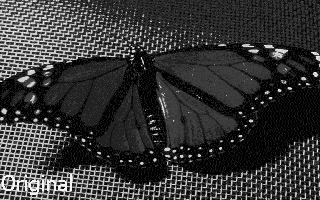
The original, unfiltered image is stored in P1. The filtered image is stored in P2. The magic starts with the variable "l" (that's an L, not a one). "l" is the pointer into Filters. Now, remember that every filter starts every 10 bytes, so if the pointer is incremented by 10 each time, you'll have a new filter every time. OK, maybe it isn't magic. Still, I'm proud of it (it didn't work the first thousand times I tried it, I'm just glad it works now). The picture is drawn (DrawPicture), a key is awaited (getch), and the filtered picture is deleted to make room for the new one. Pretty simple. Now for an explanation of the filters themselves.

There are a number of a different types of kernals used in elementary digital filtering. All of the ones I will explain are already conveniently defined in FILTER.H. Note: I am human, despite all the evidence contrary to the fact. I am capable of mistakes. If the numbers in the following sections do not match the numbers in FILTER.H, it is very likely that either set or both of them are wrong. If you notice any mistakes, I apologize. There is a great amount of numbers that can easily be mixed up.

For reference's sake, here's the original bitmap that I will digitally filter:

One of the simplest types of kernal is the low-pass spatial filter. These filters block out higher frequency pixel colors (pixels that aren't surrounded by pixels of similar color), and are used for reducing noise 1 to 2 pixels wide. Here's an example to make this more clear. Suppose you pass a low-pass spatial filter over an image where little changes. The pixels would be mostly unaffected (the lower frequency would pass through unaffected). However, let's say you pass a low-pass spatial filter over an image where there are huge changes in color that occur in small spots (there's noise). This image would be blurred and smoothed over. Images can be sharpened by subtracting and image that has been filtered with a low-pass filter from the original image. This is demonstrated in FILTLP1.CPP. Beware though, color subtraction in 256-color modes (or any mode) can make results you don't want. Here are the low-pass spatial filter kernals:

Average						LP1						LP2						LP3						Gaussian
1		1		1		1		1		1		1		1		1		1		1		1		1		2		1
1		1		1		1		2		1		1		4		1		1		12		1		2		4		2
1		1		1		1		1		1		1		1		1		1		1		1		1		2		1
9			0			10			10			12			20			20			30			16			40

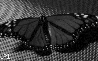
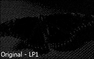
The number to the right of the normalization constant is the pointer number into Filters (FILTER.H) in which you can find the kernal. The changes in the images are subtle, but there. If you want to take a closer look, click on any of the images.

Here are the results from FILTLP1.CPP, which demonstrates color subtraction in order to produce a sharper image. The final result is indeed sharper than the original image, although the colors are skewed:

The high-pass spatial filter is used to amplify the higher-frequency aspects of an image. Higher-frequency parts of the image will become brighter, and lower-frequency parts will darken. This filter is used often to increase sharpness, but can increase noise.

High-pass spatial filters often have very large kernal centers, so that in images where there are many frequency changes, these changes are amplified and multiplied many times over. The negative coefficients are used to negate the large kernal centers. Therefore, areas of the image that have large intensity changes are intensified, while areas of the image that have little or no change are not intensified.

Mean Removal						HP1						HP2						HP3
-1		-1		-1		0		-1		0		1		-2		1		0		-1		0
-1		9		-1		-1		5		-1		-2		5		-2		-1		20		-1
-1		-1		-1		0		-1		0		1		-2		1		0		-1		0
1			50			1			60			1			70			16			80

Next : Edge Enhancement