Contents  Introduction  Preliminary discussion  Finite Element  Method  Adaptation of the  FEM  Appendix  Printable version  Discuss this article  in the forums The Series  Part 1  Part 2  Part 3 (coming soon)

The Finite Element Method (FEM)

Introduction

The efficient finite element method originates in the 1950's and with the widespread use of the digital computers has since gained considerable favour compared to other numerical approaches. This method allows to foresee stress and strain in an engineering structure, with unprecedented ease and precision. In this article, we only discuss about continuum mechanics and its applications in the FEM.

The general procedure of the finite element and conventional structural matrix method are similar. Consequently, I am going to present this method first as it easier to understand than the FEM.

Structural Matrix Method

This method allows to calculate the displacement and the stress in a structure usually made of beams. The structure is idealized as an assembly of structural members connected to one another at joints or nodes at which the resultants of the applied forces are assumed to be concentrated.

Employing the mechanics of solids or the elasticity approach, the stiffness properties of each element can be ascertained. Equilibrium and compatibility considered at each node lead to a set of algebraic equations, in which the unknowns may be nodal displacements, internal nodal forces, or both, depending upon the specific method used.

In the displacement or so-called direct stiffness method, the set of algebraic equations involves the nodal displacements. In the force method, the equations are expressed in terms of unknown internal nodal forces. A mixed method is also used, in which the equations contain both nodal displacements and internal forces.

A simple model

One of the simplest cases from the structural matrix method is to idealize each member of the structure by a spring. The stability of an elastic spring is characterized by its constant of rigidity . This constant is used to calculate the return force .

Spring fixed at its base

The relation linking displacement and force is:

is the relative length variation of the spring.

When two axial forces are applied to the spring, the stability commands that:

are respectively the forces and the displacements for each node.

Axial forces applied to the spring

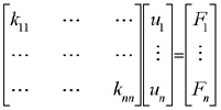
A matrix relation could replace these equations:

The matrix, which links the force vector and the displacement vector, is called the stiffness matrix of the spring.

We could assemble several elements modelized with springs to construct more complex structures, like this following example.

Structure made of three spring-elements

After assembling the three stiffness matrices of the element, a linear relation that links the forces and the displacement is found:

S is the section of the element E is the Young modulus of the material

Notice that the problem has 6 unknowns (3 nodes free along the x and the y axes), which are organized in the vector.

To resolve the problem, we apply boundary conditions: the nodes 1 and 3 are fixed in the three directions. After resolving the displacements of the node 2, the reaction forces, which are applied on the nodes 1 and 3, are found.

Refer to the bibliography for more information about the structural matrix method.

General relation

The fundamental relation that must be remembered is the matrix relation . As we are going to see, with the finite element method, theses relations could be computed for any continuous body and so not only for structures.

Principles of the FEM

In contrast in the foregoing approaches, in the finite element method, the solid continuum is divided into a finite number of elements, connected not only on their nodes, but along the hypothetical inter-element boundary as well. In addition therefore to nodal compatibility and equilibrium, as in conventional structural analysis, it is clear that compatibility must also be met along the boundaries between the elements. Because of this, the element stiffness can only be approximately determined in the finite element method.

As in the structural analyses previously cited, there are several approaches for the FEM. In this article, we treat only the commonly employed finite element displacement approach.

Theory

Let us take a stress analysis problem for a body under certain loading conditions.

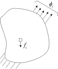
Problem characterized by its geometry, its force loading and its boundary conditions

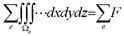
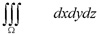
The normal analytical procedure would involve taking an extremely small box element of dimensions (dx, dy, dz) each tending to zero and then writing down the equations of equilibrium and compatibility for this element.

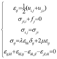
Then we would try to obtain a solution for the stress distribution in the body under the specified boundary conditions using the integration techniques over the entire body. The drawback of this method is that for complicated bodies it will be very difficult and sometimes impossible to carry out the integration procedure over the entire body.

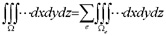
The solution to such problems can be obtained very effectively and to a high degree of accuracy using Finite Element Method. Instead of assuming a displacement field for the entire body, we divide the body into smaller elements and assume a displacement field for these individual elements. The original body or structure is then considered as an assemblage of these elements. Once again, these elements are connected to each other at joints called nodes or nodal points to form the entire structure. These individual elements are now analysed. Instead of carrying out integration over the entire body consisting of infinite number of elements of infinitesimally small dimensions, we carry out summation over the body consisting of finite number of elements of finite dimensions. By this iterative approach, the method can be effectively implemented in a computer program.

The equations of equilibrium for the entire structure or body are then obtained by combining the equilibrium equation of each element so that the continuity is ensured at each node. The necessary boundary conditions are then imposed and the equations of equilibrium are solved to obtain the required variables such as stress, strain, temperature, distribution or velocity flow depending on the application.

	Boundary Conditions
	Algebraic equations

The solution, divide to rule

We must also realize that FEM is a numerical technique and the answers obtained are not the exact solutions but only approximate. However by using appropriate procedures and proper computing facilities, we can obtain an extremely high degree of accuracy which is very much acceptable in practice. Notice that the "acceptable" term is used for engineering problems. In the video games field, after using acceptable procedures, the result can be considered physically correct.

	Physical system
	Equations with partial derivatives
	Integral formulation
Analytical method		FEM
? Difficulty to carry out the integration procedure		Systems of algebraic equations
		Approximate Solution

Consequently, the structural matrix method is very close to the FEM. Actually the divided structures of beams are replaced by continuum solids.

Stiffness matrix

Previously, the stiffness matrix of a spring has been examined above. The finite element method works with more complicated element in two or three dimensions.

Example of finite elements (from An Introduction of the finite elements by Dhatt and Touzot)

In the project, the only used element is a cube made of eight nodes with three degrees of freedom by nodes. In fact, each node could move along the x, y and z axes. In the previously example with the spring, the nodes located at each extremities of the element can move only along the axe of the spring.

The cubic element used for the project

Three degrees of freedom by node

Consequently, the dimension of the stiffness matrix of this element is 24 by 24:

The matrix depends only on the material properties and dimensions of the cube. The analytical form has been calculated with Maple. The result can be found here. Moreover, the Maple file is downloadable here.

Refer to bibliography to know how to compute stiffness matrices.

Common applications of the finite elements method

FEM has a wide range of applications as follows:

• Stress Analysis;
• Heat Transfer;
• Fluid Flow;
• Torsion Analysis;
• etc.

Some pictures, showing the capabilities of this method, follow.

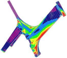
Stress in the frame of a bike

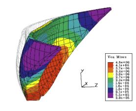
Deformation of a dam

In this article, I will demonstrate that it is possible to adapt these industrial cases for the video games. These potential cases follow below:

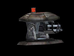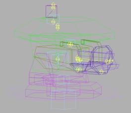
Turret (from Half-Life SDK)

Next : Adaptation of the FEM