II – Matrix convolution filters
1 – Definition, properties and speed
a – Definition and a bit of theory
Let us first recall a basic principle in signal processing theory: for audio signals for example, when you have a filter (or any kind of linear system) you can compute its response to an entering signal x(t) by convolving x(t) and the response of the filter to a delta impulse: h(t), you then have:
Continuous time:

(R11)
Discrete time:

(R12)
If you are not familiar with this technique and don't want to get bored, you can skip this section which is not crucial to understand the following algorithms. In the same way that we can do for one-dimensional convolution, we can also compute image convolutions, and basically this is what matrix convolution is all about. The difference here is obviously that we are dealing with a two dimensions object: the bitmap. Likewise audio signal, a bitmap can be viewed as a summation of impulses, that is to say scaled and shifted delta functions. If you want to know the output image of a filter, you will simply have to convolve the entering bitmap with the bitmap representing the impulse response of the image filter. The two dimensional delta functions is an image composed by all zeros, except for a single pixel, which has value of one. When this delta function is passed through a linear system, we will obtain a pattern, the impulse response of this system. The impulse response is often called the 'Point spread function' (PSF). Thus convolution matrixes, PSF, filter impulse response or filter kernel represent the same thing. Two dimensional convolution works just like one dimensional discrete convolutions, the output image y of an entering bitmap x, through a filter system of bitmap impulse response h (width and height M) is given by formula:
(R13)
Notice that the entering signal (Or the impulse response) alike one dimensional signals must first be flipped left for right and top for bottom before being multiplied and summed: this is explained by the (k-i) index in the sums of (R12); and by the (r-j) and (c-i) indexes in (R13). Most of the time we will deal with symmetrical filters, therefore these flips have no effect and can be ignored; keep in mind that for non symmetrical signals we will need to rotate h before doing anything. By the way two dimensional convolutions is also called matrix convolution.
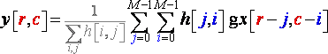
The presence of a normalising factor in gray in formula (R13), can be explained by the fact that we want y[r,c] to be found between 0 and 255. Therefore we can say that computing y[r,c] is like computing the center of gravity of some x[i,j] color values affected by the weights in the filter matrix. This normalising factor is sometimes included into the filter matrix itself, sometimes you have to add it yourself. Just remember to always check that the numbers possible to obtain with y[r,c] are always between 0 and 255.
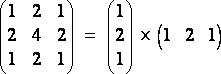
Let us have an example of matrix convolution:
Figure 5: Matrix Convolution
There are numerous types of matrix filters, smoothing, high pass, edge detection, etc… The main issue in matrix convolution is that it requires an astronomic number of computations. For example is a 320x200 image, is convolved with a 9x9 PSF (Pulse spread function), we already need almost six millions of multiplications and additions (320x200x9x9). Several strategies are useful to reduce the execution time when computing matrix convolutions:
- Reducing the size of the filter reduces as much the execution time. Most of the time small filters 3x3 can do the job perfectly.
- Decompose the convolution matrix of the filter into a product of an horizontal vector and a vertical vector: x[r,c] = vert[r] x horz[c]. In which case we can convolve first all the horizontal lines with the horizontal vector and then convolve the vertical line with the vertical vector. Vert[r] and horz[c] are the projections of the matrix on the x and y axis of the bitmap. You can generate an infinity of seperable matrixes filters by choosing a vert[r] and a horz[c] and multiplying them together. This is a really efficient improvement because it brings the global complexity from N²M² to N²M (where N is the number of rows and columns of the input bitmap and M that of the matrix filter).
- Last method is FFT convolution. It becomes really useful for big matrix filters that cannot be reduced. Indeed Convolution in time or space domain is equivalent to multiplying in frequency domain. We will study in detail this method in the last part of this chapter.
1 – A few common filters
a – sharpness filter
Let us have some examples of different filter kernels. The first one will be the sharpness filter. Its aim is to make the image look more precise. The typical matrix convolution for a sharpness filter is:
(R14)
Looking at those matrixes you can feel that for each pixel on the source image we are going to compute the differences with its neighbors and make an average between those differences and the original color of the pixel. Therefore this filter will be enhancing the edges. Once you have understood how to compute a matrix convolution the algorithm is easy to implement:
Algorithm 7 : Sharpness filter
- For every pixel ( i , j ) on the output bitmap
- Compute its color using formula (R13)
- Set the pixel
#define sharp_w 3
#define sharp_h 3

sumr=0;
sumg=0;
sumb=0;

int sharpen_filter[sharp_w][sharp_h]={{0,-1,0},{-1,5,-1},{0,-1,0}};
int sharp_sum=1;

for(i=1;i<temp->w-1;i++){
  for(j=1;j<temp->h-1;j++){
    for(k=0;k<sharp_w;k++){
      for(l=0;l<sharp_h;l++){

        color=getpixel(temp,i-((sharp_w-1)>>1)+k,j-
          ((sharp_h-1)>>1)+l);
        r=getr32(color);
        g=getg32(color);
        b=getb32(color);
        sumr+=r*sharpen_filter[k][l];
        sumg+=g*sharpen_filter[k][l];
        sumb+=b*sharpen_filter[k][l];
      }
    }

    sumr/=sharp_sum;
    sumb/=sharp_sum;
    sumg/=sharp_sum;

    putpixel(temp1,i,j,makecol(sumr,sumg,sumb));
  }
}
Unfortunately this filter is not separable and we cannot decompose the filter matrix in the product of a vertical vector and a horizontal vector. The global complexity of the algorithm is N²M² where and N and M are the dimensions of the filter bitmap and of the source bitmap. This algorithm much slower than any of the others we have studied up to now. Use it carefully.
Picture 9: Sharpness filter effects
b – Edge Detection
This algorithm uses matrix convolution to detect edges. I found it much slower than the algorithm seen in the first part for an equivalent result. Here are matrix filters exemples for edge detection:
(R15)
The kernel elements should be balanced and arranged to emphasize differences along the direction of the edge to be detected. You may have noticed that some filters emphasize the diagonal edges like the third one, while others stress horizontal edges the fourth and the second. The first is quite efficient because it takes into account edges in any direction. As always, you must choose the filter the most adapted to your problem.
A second important point: notice that the sum of the filter matrix coefficients we usually used as a normalising factor in (R13) is null. Two things to do: we will avoid dividing by zero, we will add to the double sums the value of 128 to bring the color value y[r,c] back into 0-255. The complexity of the algorithm doesn't change N²M².
Algorithm 8 : Edge Detection Filter
- For every pixel ( i , j ) on the output bitmap
- Compute its color using formula (R13)
- Set the pixel
#define edge_w 3
#define edge_h 3
sumr=0;
sumg=0;
sumb=0;
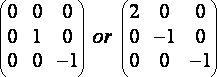
int edge_filter[edge_w][edge_h]={{-1,-1,-1},{-1,8,-1},{-1,-1,-1}};
int edge_sum=0; // Beware of the naughty zero
for(i=1;i<temp->w-1;i++){
for(j=1;j<temp->h-1;j++){
for(k=0;k<edge_w;k++){
for(l=0;l<edge_h;l++){
color=getpixel(temp,i-((edge_w-1)>>1)+k,j-((edge_h-1)>>1)+l);
r=getr32(color);
g=getg32(color);
b=getb32(color);
sumr+=r*edge_filter[k][l];
sumg+=g*edge_filter[k][l];
sumb+=b*edge_filter[k][l];
}
}
sumr+=128;
sumb+=128;
sumg+=128;
putpixel(temp1,i,j,makecol(sumr,sumg,sumb));
}
}
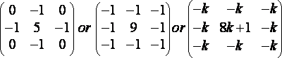
c – Embossing filter
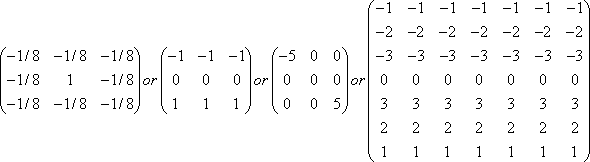
The embossing effect gives the optical illusion that some objects of the picture are closer or farther away than the background, making a 3D or embossed effect. This filter is strongly related to the previous one, except that it is not symmetrical, and only along a diagonal. Here are some examples of kernels:
(R16)
Here again we will avoid dividing by the normalising factor 0, and we will add 128 to all the double sums to get correct color values. The implementation of this algorithm is just the same as the prvious one except that you must first convert the image into grayscale.
Algorithm 9 : Embossing effect filter
- Convert the image into grayscale
- For every pixel ( i , j ) on the output bitmap
- Compute its color using formula (R13)
- Set the pixel
#define emboss_w 3
#define emboss_h 3

sumr=0;
sumg=0;
sumb=0;

int emboss_filter[emboss_w][emboss_h]={{2,0,0},{0,-1,0},{0,0,-1}};
int emboss_sum=1;

for(i=1;i<temp->w-1;i++){
  for(j=1;j<temp->h-1;j++){
    color=getpixel(temp,i,j);
    r=getr32(color);
    g=getg32(color);
    b=getb32(color);
    h=(r+g+b)/3;
    if(h>255)
      h=255;
    if(h<0)
      h=0;
    putpixel(temp1,i,j,makecol(h,h,h));
  }
}

for(i=1;i<temp->w-1;i++){
  for(j=1;j<temp->h-1;j++){
    sumr=0;
    for(k=0;k<emboss_w;k++){
      for(l=0;l<emboss_h;l++){
        color=getpixel(temp1,i-((emboss_w-1)>>1)+k,j-((
        emboss_h-1)>>1)+l);
        r=getr32(color);
        sumr+=r*emboss_filter[k][l];
      }
    }
    sumr/=emboss_sum;
    sumr+=128;
    if(sumr>255)
      sumr=255;
    if(sumr<0)
      sumr=0;
    putpixel(temp2,i,j,makecol(sumr,sumr,sumr));
  }
}
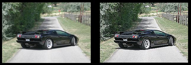
Here are the effects of
this algorithm:
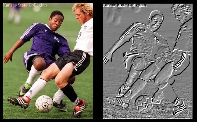
Picture 9: Embossing filter
d – Gaussian blur filter
As its name suggests, the Gaussian blur filter has a smoothing effect on images. It is in fact a low pass filter. Apart from being circularly symmetric, edges and lines in various directions are treated similarly, the Gaussian blur filters have very advantageous characteristics:
- They are separable into the product of horizontal and vertical vectors.
- Large kernels can be decomposed into the sequential application of small kernels.
- The rows and columns operations can be formulated as finite state machines to produce highly efficient code.
We will only study here the first optimisation, and leave the last two to a further learning (you can find more information on these techniques in the sources of this paper). So, the filter kernel of the Gaussian blur filter is decomposable in the product of a vertical vector and an horizontal vector, here are the possible vectors, multiplied by each other they will produce gaussian blur filters:
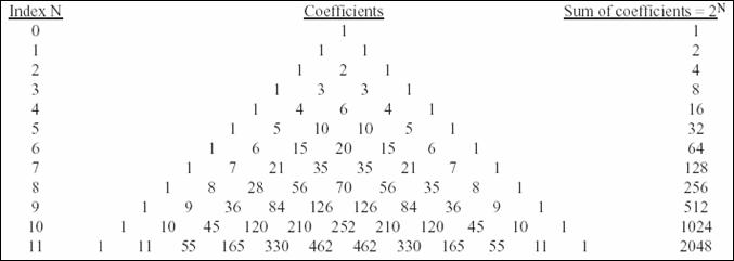
Figure 6: Gaussian filters coefficients
(source: An efficient algorithm for gaussian blur filters, by F. Waltz and W. Miller)
Gaussian blur filter kernel example (order 2):
(R17)
What increases greatly the algorithm's speed compared to the previous 'brute force' methods is that we will first convolve rows of the image with the (1 2 1) vector and then the columns of pixels with the (1 2 1)T vector. Thus we will use an intermediary bitmap where will be stored the results of the first convolutions. In the final bitmap will be stored the output of the second stage convolutions. So here is the algorithm with an order 6. The fact that we separated our matrix in a product of vectors, ports the complexity of the algorithm to N²M where M is the size of the filter and N that of the source bitmap. Therefore for a order 6 filter we have 6 times less elementary operations. The result is quite satisfying; on my computer I obtained the equivalent transform rate of the order 3 filters we have seen before. We have thus reached the speed of order 3 filters but with the quality result of an order 6!
Algorithm 10 : Gaussian blur implementation
- For every pixel ( i , j ) on the intermediate bitmap
- Compute its color using formula (R13), source bitmap pixels and horizontal vector of the matrix decomposition (eg : (1 2 1))
- Set the pixel on the intermediate bitmap
- For every pixel ( i, j ) on the output bitmap
- Compute its color using formula (R13), intermediate bitmap pixels and vertical vector of the matrix decomposition (eg : (1 2 1)T)
- Set the pixel on the output bitmap
#define gauss_width 7

sumr=0;
sumg=0;
sumb=0;

int gauss_fact[gauss_width]={1,6,15,20,15,6,1};
int gauss_sum=64;

for(i=1;i<temp->w-1;i++){
  for(j=1;j<temp->h-1;j++){
    sumr=0;
    sumg=0;
    sumb=0;
    for(k=0;k<gauss_width;k++){
      color=getpixel(temp,i-((gauss_width-1)>>1)+k,j);
      r=getr32(color);
      g=getg32(color);
      b=getb32(color);
      sumr+=r*gauss_fact[k];
      sumg+=g*gauss_fact[k];
      sumb+=b*gauss_fact[k];

    }
    putpixel(temp1,i,j,makecol(sumr/gauss_sum,sumg/gauss_sum,
      sumb/gauss_sum));
  }
}

for(i=1;i<temp->w-1;i++){
  for(j=1;j<temp->h-1;j++){
    sumr=0;
    sumg=0;
    sumb=0;
    for(k=0;k<gauss_width;k++){
      color=getpixel(temp1,i,j-((gauss_width-1)>>1)+k);
      r=getr32(color);
      g=getg32(color);
      b=getb32(color);

      sumr+=r*gauss_fact[k];
      sumg+=g*gauss_fact[k];
      sumb+=b*gauss_fact[k];
    }
    sumr/=gauss_sum;
    sumg/=gauss_sum;
    sumb/=gauss_sum;

    putpixel(temp2,i,j,makecol(sumr,sumg,sumb));
  }
}

Picture 10: Gaussian blur filter effects
1 – FFT enhanced convolution
a – FFT with bitmaps
There is a major difference between the use of Fast Fourier Transform in audio signal and in image data. While in the first one fourier analysis was a way to trasform the confusing time domain data into an easy to understand frequency spectrum; the second one converts the straight forward information in spatial domain to a scrambled form in the frequency domain. Therefore, in audio analysis, FFT was a way to 'see' and 'understand' more clearly the signal: now in image processing, FFT messes up the information in an unreadable coding. We will not be able to use FFT in Digital image processing to design filters or to analyse data. Image filters are normally designed in the spatial domain, where the information is encoded in its simplest form. We will always prefer the appelations 'smotthing' and 'shapening' to 'low pass' or 'high pass filter'.
However, some principles of the FFT are still true and very useful in digital image processing: Convolving two functions is equivalent to multiplying in the frequency domain their FFT and then computing an inverse FFT to obtain the resulting signal. The second useful property of the frequency domain is the Fourier Slice Theorem, this therorem deals with the relationship between an image and its projections (the image viewed from its sides. We won't study this theorem here: it would take us far away from our concerns. Let's come back to image convolution using a FFT.
The FFT of an image is very easy to compute once you know how to do one dimensional FFTs (just like in the audio signal). First, if the dimensions of the image are not a power of two we wiil have to increase its size by adding zero pixels; the image must become NxN sized, where N is a power of 2 (32, 64, 128, 256, 1024 …). The two dimensional array that holds the image will be called the real array, and we will use another array of the same dimensions, an imaginary array. To compute the FFT of the image we will take the one-dimensional FFT of each of the rows, followed by the FFT of each of the columns. More precisely, we wiil take the FFT of the N pixel values of row 0 of the real array (original bitmap), store its real part output back into row 0 of real array, and the imaginary part into row 0 of imaginary array. We will repeat this procedure from row 1 to N-1. We will obtain two intermediate images: the real array and the imaginary array. We will then start the process all over again but with columns FFT and using the intermediate images as source. That is to say, compute the FFT of the N pixel values in column 0 of the real array and of the imaginary array (making complex numbers). We will store the result back into column 0 of real and imaginary arrays. After this procedure is repeated through all the columns, we obtain the frequency spectrum of the image, its real part in the real array and its imaginary part in the imaginary array.
Since row and columns are interchangeable in an image, you can start the algorithm by computing FFT on columns followed by rows. The amplitudes of the low frequencies can be found in the corners of the real and imaginary arrays, whereas the high frequencies are close to the center of the output images. The inverse FFT is obviously calculated by taking the inverse FFT of each row and of each column. Properties of the FFT give us a last property of the output images:
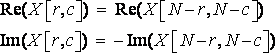
(R18)
The idea of passing to the frequency domain to compute an FFT is the following. We will pass both of the images we want to convolve into the frequency domain, adapting their dimensions so that they have both the same size, NxN power of 2, we will fill empty zones with zeros if necessary. Remember to rotate one of the images to convolve by 180° around its center before starting anything. Indeed convolution, according to its mathematical definition, flips one of the source images. Therefore we will have to compensate it by rotating of of the images first. Once we have the real and imaginary arrays FFT outputs for the two source images, we will multiply each of the real values and imaginary values of one image with each of the real values and imaginary values of the other, this will give us our final image in the frequency domain. Finally we compute the inverse FFT of this final image and we obtain X1 convolved with X2. On the following page you will find in figure 7 the process explained in detail.
The convolution by FFT becomes efficient for big kernels (30x30), and you may notice that its execution time doesn't depend on the kernel's size but on the image's size. Standard convolution's execution time depends on both the kernel size and the source image size. Figure 8 is a graph of the execution time for computing convolutions with different kernel sizes and for two sizes of image (128x128 and 512x512), using FFT, standard floating point convolution (FP) and standard integer convolution (INT).
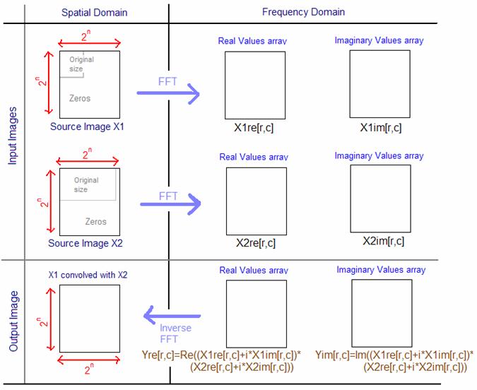
Figure 7: The FFT way of convolving two images
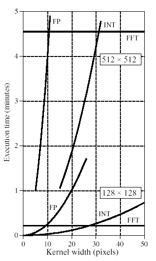
Figure 8: Computing time for different convolution methods and for different kernel sizes
(source: The scientist and engineer's guide to Digital Signal Processing, by Steven W. Smith))

Examples of application
|
|