III Examples of application
1 Motion Detection and Tracking
a Static and Dynamic backgrounds
The aim of motion detection is to detect in a streaming video source, which we will consider as a very rapid succession of bitmaps, the presence of moving objects and to be able to track their position. Motion detection in surveillance systems is rarely implemented with software means because it is not trustable enough and good systems remain very expensive, companies usualy prefer hiring surveillance employees. However, video motion detection does exist and works pretty well as long as you know exactly what you want to do. Are you going to have a static background? Is the camera going to move around? Do you want to spot exclusively living entities? Do you know in advance the object which going to move in the camera's field? Lots of questions we will have to answer before making our choices for the algorithm used.
There are two major types of motion detection: static background motion detection and dynamic background motion detection. The first will be used for surveillance means: the surveillance camera doesn't move and has a capture (in a bitmap for example) of the static background it is facing. The second is much more complex. Indeed in the entering streaming video the background moves at the same time as moving objects we want to spot, all the issue consists in seperating the object from the background. Therefore we will make a major hypothesis: the object moves much slower than the background.
b Static background motion detection
Let us suppose a video camera is facing a static background. The static image of this background, say, when no object is in the field of the camera, is stored in a bitmap. The idea is very simple. When surveillance is turned on, for each frame received (or every n frames, depending on the framerate of the recording system and on the relative speed of the potential target objects) the software compares each pixel of the frame with those of the static background image. If a pixel is very different it is marked as white, if not it is left in black. We will calculate the 'difference' between these two pixels by calculating the distance between them with (R1), and comparing it to a threshold value. Some techniques set this threshold value according to the number of color the arriving frame contains, I haven't tested this technique personally but it seems fairly wise. Therefore after this stage, the suspected moving objects are marked in white pixels, while the background is all set to black. Unfortunately, lights reflections, hardware imperfections, other unpredictable factors, will introduce some parasitical white pixels which don't correspond to real objects moving. We will try to remove those isolated white pixels to purify the obtained image.
Thus we will pass the resulting black and white image through an aliasing filter, which is meant to remove noise. This filter will remove all the isolated noisy white pixels and leave, if there are, the big white zones corresponding to moving objects. Basically we scan the image with a window of NxN pixels (depends on the size of the frames), if the center of the pixel of the NxN square is white, and less than K pixels in the window are set to white then it is set back to black because it is probably just an isolated noise not corresponding to a concrete object moving. Oppositly if more than K pixels are set to white and the center pixel is white we leave it as it is. However, this requires a lot of pixel scanning N²M², where M is the dimension of the frames; therefore we will rather scan the image by squares of NxN, for each of them count the number of white pixels they contain, if it superior to the treshhold value the whole NxN square is set to white on the bitmap else we set it black, we then jumps to the next NxN square. With this technique we limit the pixels access to M² which is a lot better. The output image will seem very squary but this is not a problem.
At that point we should have a black image with perhaps some white zones corresponding to moving objects in the fields of the camera. Thus we can already answer to the basic question: is there a moving object in the camera's field? A simple test on the presence of white pixels on the image will answer. Here is an example stage by stage of the processing:
Picture 10: The static background image of the camera's field
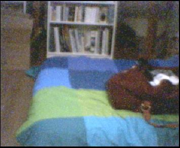
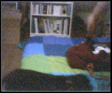
Picture 11: My dog (yes, the weird shape in black) has jumped on the bed to look if there isn't something to eat in the red bag
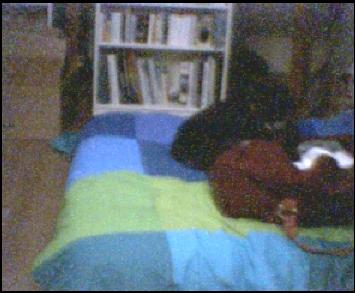
Picture 12: After comparing each pixel of the current frame with the static background we already have a good idea of the moving shape. Notice all the noise (small isolated pixels in white) due to the poor quality of my webcam. The fact that my dog is searching in the bag makes it move a little, which is also detected on the right of the image.

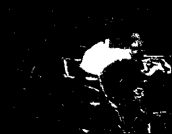
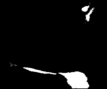
Picture 13: The aliasing filter has removed all the noise and parasites. We finally isolated the moving shape and we are now capable of giving its exact position, width, height etc
c Unknown background (dynamic) motion detection
The case of unknown background motion detection is pretty similar to the previous situation. This becomes useful when you cannot predict the background of the camera's field and therefore cannot apply the previous algorithm. Notice that we will not study here, the motion detection algorithms in which the camera is moving permanently. Here the camera doesn't actually move, nor does it use a background reference like just before. Instead of comparing each received frame to a reference static background we are going to compare the frames received together. This technique is known as frame differentiating.
This is how the algorithm works on a streaming source of frames coming from a video camera: We will store a received frame in bitmap A, wait for the next n frames to pass without doing anything, capture the n+1 frame, compare it to A, store the n+1 frame in A, wait for n frames to pass, capture the 2n+2 frame, compare to A, store in A, and so on. Therefore we will regularly compare two frames together, seperated by n other frames that we will simply loose. This n value, the comparison rate, must be low enough not to miss some moving objects which would go right through the camera's field, but it also must be high enough to see differences between frames if a very slow object is moving in the camera's field. For the example of my webcam and my dog, I took n=10, with a streaming frame rate of 30 fps, this corresponds to 1/3 secs.
When we compare the two frames together we use the same method as seen above, if a pixel changes a lot of color from one frame to another we set it as white, else we leave it in black. We then make the resulting image pass through an aliasing filter and finally we are able to spot the moving objects.
Obviously this technique is less precise than the previous one because we don't spot directly the moving object in itself but we detect the changing zones in the frames and assimilate those changing zones to a part of background which has been recovered recently by a part of the object. Therefore we will only see edges of moving objects. Here is an example of results:
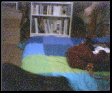
Picture 14: One of the frames we are going to compare (bitmapA)
Picture 15: The second frame to compare, we have skipped 10 frames ever since we saved bitmapA. Therefore the dog has had the time to move and we will see a difference between the frames.
Picture 15: The algorithm sees the zones which have changed colors: corresponding to the head of the dog walking and to my hand I was agitating.

Picture 16: After the aliasing filter only the main zones are left and enable us to situate roughly the moving objects on the camera's field.
1 Shape recognition
a Shape recognition by convolution
The aim of shape recognition is to make the computer recognize particular shapes or patterns in a big source bitmap. Like the audio signal with speech recognition, this is far from beeing a trivial issue. Lots of powerful but also very complex methods exist to recognize shapes in an image. The one we are going to study here is very basic and makes a number of assumptions to work correctly. The shape we are going to try to situate on a source image must not be rotated nor distorted on this actual image. This limits a lot the use of this algorithm because in real situations the pattern you search in an image is always a bit rotated or distorted. In one dimensional signal correlation between two signals quantifies how similar they are; in two dimensions the principle is the same. Computing the correlation of the source image and the pattern we are looking for while give us an output image with a peak of white corresponding to the position of the pattern in the image. In fact we make our source image pass through a filter which kernel is the pattern we are looking for. When computing the output image pixel by pixel at one point the kernel and the position of the searched pattern in the image will correspond perfectly, this will give us a peak of white we will be able to situate.
Therefore the implementation of the algorithm is very simple; we compute the matrix convolution of the source image with the kernel, constituted of the pattern we want to search. In this case you will almost be forced to use the FFT convolution, indeed the searched patterns are often more then 30 pixels large, and for kernels of over 30x30 it's faster to use an FFT rather than straight convolution. I tried this algorithm without the FFT optimization and it is very very slow: about one transform per minute!
However the results themselves are quite remarkable, the position of the pattern is well recognized, sometimes with a bit of noise though. A nice way to enhance the results and make the peaks even more precise is to make the kernel pass through an edge enhancement filter; this will make the kernel more selective and precise. Here are the results of the algorithm:
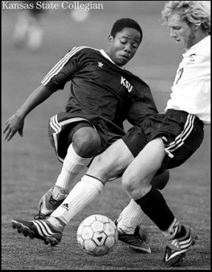
Picture 17: Our source image: will you find the ball before the computer does?

Picture 18: The pattern the algorithm will be looking for.
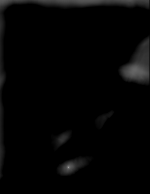
Picture 19: The white peak corresponding to the ball's position.
Picture 20: Another source image.

Picture 21: The pattern the algorithm will be looking for.
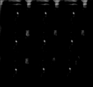
Picture 22: The white peak corresponds to the positions of the patterns.
Conclusion
Digital image processing is far from being a simple transpose of audio signal principles to a two dimensions space. Image signal has its particular properties, and therefore we have to deal with it in a specific way. The Fast Fourier Transform, for example, which was such a practical tool in audio processing, becomes useless in image processing. Oppositely, digital filters are easier to create directly, without any signal transforms, in image processing.
Digital image processing has become a vast domain of modern signal technologies. Its applications pass far beyond simple aesthetical considerations, and they include medical imagery, television and multimedia signals, security, portable digital devices, video compression, and even digital movies. We have been flying over some elementary notions in image processing but there is yet a lot more to explore. If you are beginning in this topic, I hope this paper will have given you the taste and the motivation to carry on.
Sources and Links
Appendix A : Last minute adds
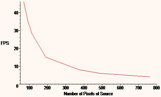
Figure 9: Plot of the Tranforms per second with the color extraction algorithm according to the number of pixels of the source bitmap (/1000). It is fair to conclude that the fps decrease in an hyperbolic way with the number of pixels in the source bitmap. Notice also that it doesn't have anything to do with the complexity of the algorithm which is a straight according to the number of pixels (a*N²).
|