sponsors gamedev.net search:

Geomorphing in Hardware Doing geomorphing for a single patch basically means doing vertex tweening between the current tessellation level and the next finer one. The tessellation level calculation returns a tessellation factor in form of a floating point value where the integer part means the current level and the fractional part denotes the tweening factor. E.g. a factor of 2.46 means that tweening is done between levels 2 and 3 and the tweening factor is 0.46. Tweening between two mesh representations is a well known technique in computer graphics and easily allows an implementation of morphing for one single patch (vertices that should not move simply have the same position in both representations). The problem becomes more difficult if a patch's neighbors are considered. Problems start with the shared border vertices which can only follow one of the two patches but not both (unless we accept gaps). As a consequence one patch has to adapt its border vertices to those of its neighbor. In order to do correct geomorphing it is necessary that the finer patch allows the coarser one to dictate the border vertices' position. This means that we do not only have to care about one tweening factor as in the single patch case but have to add four more factors for the four shared neighbor vertices. Since the vertex shader can not distinguish between interior and border vertices these five factors have to be applied to all vertices of a patch. So we are doing a tweening between five meshes. As if this wasn't already enough, we also have to take special care of the inner neighbor vertices of the border vertices. Unfortunately these vertices also need their own tweening factor in order to allow correct vertex insertion (when switching to a finer tessellation level). To point out this quite complicated situation more clearly we go back to the example of figure 6b. For example we state that the patch's left border follows its coarser left neighbor. Then the tweening factor of vertex '1' is depends on the left neighbor, whereas the tweening factor of all interior vertices (such as vertex '2') depend on the patch itself. When the patch reaches its next finer tessellation level (figure 6a), the new vertex 'A' is inserted. Figure 9 shows the range in which the vertices '1' and '2' can move and the - in this area lying - range in which vertex 'A' has to be inserted. (Recall that a newly inserted vertex must always lie in the middle of its preexisting neighbors). To make it clear why vertex 'A' needs its own tweening factor suppose that the vertices '1' and '2' are both at their bottom position when 'A' is inserted (tweeningL and tweeningI are both 0.0). Later on when 'A' is removed the vertices '1' and '2' might lie somewhere else and 'A' would now probably not lie in the middle between those two if it had the same tweening factor as vertex '1' or vertex '2'. The consequence is that vertex 'A' must have a tweening factor (tweeningA) which depends on both the factor of vertex '1' (tweeningL - the factor from the left neighboring patch) and on that of vertex '2' (tweeningI - the factor by that all interior vertices are tweened). Figure 9: Vertex insertion/removal range What we want is the following: Vertex 'A' should be inserted/removed in the middle between the positions of Vertex '1' and Vertex '2' not pop when the patch switches to another tessellation level not pop when the left neighbor switches to another tessellation level. The simple formula tweeningA = (1.0-tweeningL) * tweeningI does the job. Each side of a patch has such a 'tweeningA' which results in four additional tessellation levels. Summing this up we result in having have 9 tessellation levels which must all be combined every frame for each vertex. What we actually do in order to calculate the final position of a vertex is the following: PosFinal = PosBase + tweeningI*dI + tweeningL*dL + tweeningR*dR + tweeningT*dT + … Since we only morph in one direction (as there is no reason to morph other than up/down in a heightmap generated terrain) this results in nine multiplications and nine additions just for the geomorphing task (not taking into account any matrix multiplications for transformation). This would be quite slow in terms of performance doing it on the CPU. Fortunately the GPU provides us with an ideal operation for our problem. The vertex shader command dp4 can multiply four values with four other values and sum the products up in just one instruction. This allows us to do all these calculations in just five instructions which is only slightly more than a single 4x4 matrix multiplication takes. The following code snippet shows the vertex data and constants layout that is pushed onto the graphics card. ; Constants specified by the app ; ; c0 = (factorSelf, 0.0f, 0.5f, 1.0f) ; c2 = (factorLeft, factorLeft2, factorRight, factorRight2), ; c3 = (factorBottom, factorBottom2, factorTop, factorTop2) ; ; c4-c7 = WorldViewProjection Matrix ; c8-c11 = Pass 0 Texture Matrix ; ; ; Vertex components (as specified in the vertex DECLARATION) ; ; v0 = (posX, posZ, texX, texY) ; v1 = (posY, yMoveSelf, 0.0, 1.0) ; v2 = (yMoveLeft, yMoveLeft2, yMoveRight, yMoveRight2) ; v3 = (yMoveBottom, yMoveBottom2, yMoveTop, yMoveTop2) We see that only four vectors are needed to describe each vertex including all tweening. Note that those vectors v0-v3 do not change as long as the patch is not retessellated and are therefore good candidates for static vertex buffers. The following code shows how vertices are tweened and transformed by the view/projection matrix. ;------------------------------------------------------------------------- ; Vertex transformation ;------------------------------------------------------------------------- mov r0, v0.xzyy ; build the base vertex mov r0.w, c0.w ; set w-component to 1.0 dp4 r1.x, v2, c2 ; calc all left and right neighbor tweening dp4 r1.y, v3, c3 ; calc all bottom and top neighbor tweening mad r0.y, v1.y, c0.x, v1.x ; add factorSelf*yMoveSelf add r0.y, r0.y, r1.x ; add left & right factors add r0.y, r0.y, r1.y ; add bottom & top factors m4x4 r3, r0, c4 ; matrix transformation mov oPos, r3 While this code could surely be further optimized there is no real reason to do so, since it is already very short for a typical vertex shader. Finally there is only texture coordinate transformation. ;------------------------------------------------------------------------- ; Texture coordinates ;------------------------------------------------------------------------- ; Create tex coords for pass 0 - material (use texture matrix) dp4 oT0.x, v0.z, c8 dp4 oT0.y, v0.w, c9 ; Create tex coords for pass 1 - lightmap (simple copy, no transformation) mov oT1.xy, v0.zw oT0 is multiplied by the texture matrix to allow scaling, rotation and movement of materials and cloud shadows. oT1 is not transformed since the texture coordinates for the lightmap do not change and always span (0,0)-(1,1). 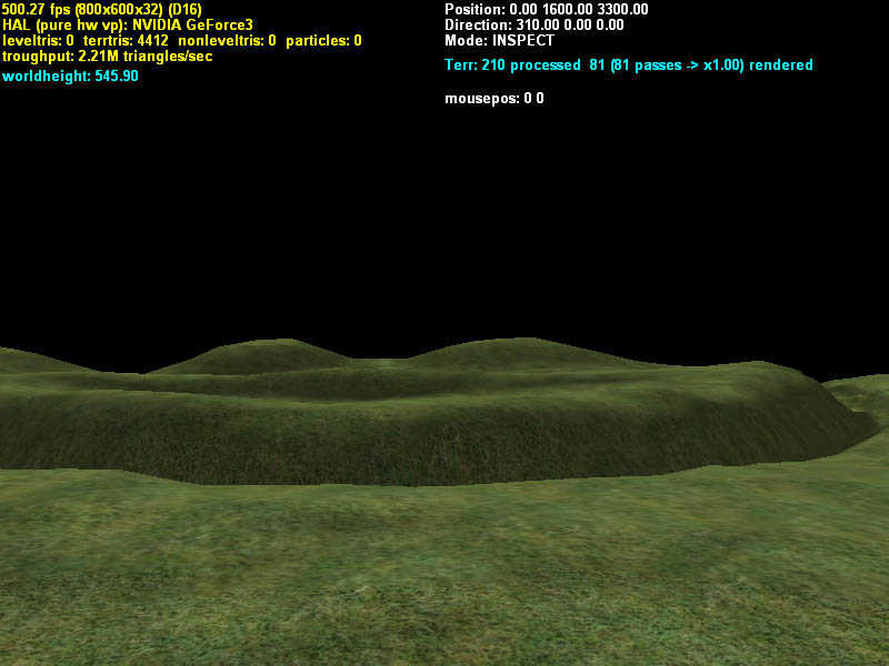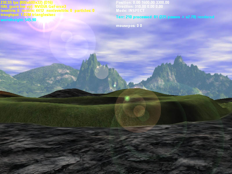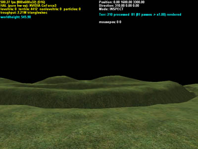Results Table 1 shows frame rates achieved on an Athlon-1300 with a standard Geforce3. The minimum scene uses just one material together with a lightmap (2 textures in one render pass - see Figure 10a). The full scene renders the same landscape with three materials plus a clouds shadow layer plus a skybox and a large lens flare (7 textures in 4 render passes for the terrain - see Figure 10b).   Static LOD Software Morphing Hardware Morphing Mininum Scene 586 fps 312 fps 583 fps Full Scene 231 fps 205 fps 230 fps Table1: Frame rates achieved at different scene setups and LOD systems. The table shows that geomorphing done using the GPU is as almost fast as doing no geomorphing at all. In the minimum scene the software morphing method falls back tremendously since the CPU and the system bus can not deliver the high frame rates (recall that software morphing needs to send all vertices over the bus each frame) achieved by the other methods. Things change when using the full scene setup. Here the software morphing takes advantage of the fact that the terrain is created and sent to the GPU only once but is used four times per frame for the four render passes and that the skybox and lens flare slow down the frame rate independently. Notice that the software morphing method uses the same approach as for hardware morphing. An implementation fundamentally targeted for software rendering would come off far better. In this article I've shown how to render a dynamically view-dependently triangulated landscape with geomorphing by taking advantage of today's graphics hardware. Splitting the mesh into smaller parts allowed us to apply the described optimizations which lead to achieved high frame rates. Further work could be done to extend the system to use geometry paging for really large terrains. Other open topics are the implementation of different render paths for several graphics card or using a bump map instead of a lightmap in order to achieve dynamic lighting The new generation of DX9 cards allows the use of up to 16 textures per pass which would enable us to draw seven materials plus a cloud shadow layer in just one pass. Sample Shots Click onto images to enlarge. 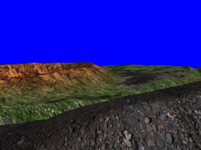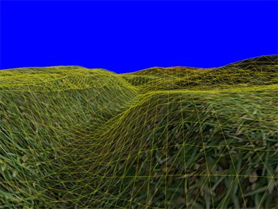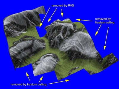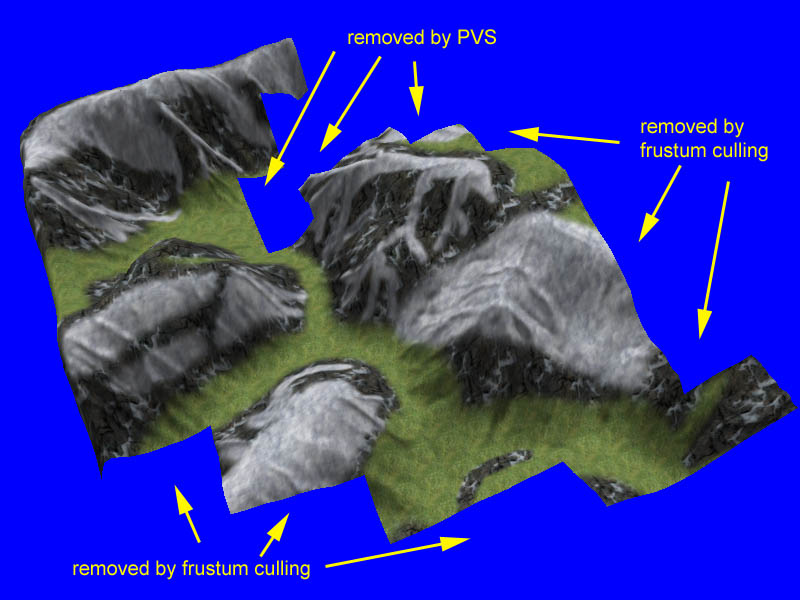Figure 10a: Terrain with one material layer Figure 10b: Same 10a but with three materials (grass, stone, mud) + moving cloud layer + skybox + lens flare       Figure 10c: Terrain with overlaid triangle mesh Figure 10d: Getting close to the ground the highly detailed materials become visible       Figure 10e: View from the camera's position Figure 10f: Same scene as 10e from a different viewpoint with same PVS and culling performed References [Air91] John Airey, "Increasing Update Rates in the Building Walkthrough System with Automatic Model-Space Subdivision and Potentially Visible Set Calculations", PhD thesis, University of North Carolina, Chappel Hill, 1991. [Boe00] Willem H. de Boer, "Fast Terrain Rendering Using Geometrical MipMapping" E-mersion Project, October 2000 (http://www.connectii.net/emersion) [Cor01] Corel Bryce by Corel Corporation (http://www.corel.com) [Duc97] M. Duchaineau, M. Wolinski, D. Sigeti, M. Miller, C. Aldrich, M. Mineev-Weinstein, "ROAMing Terrain: Real-time Optimally Adapting Meshes" (http://www.llnl.gov/graphics/ROAM), IEEE Visualization, Oct. 1997, pp. 81-88 [Eva96] Francine Evans, Steven Skiena, and Amitabh Varshney. Optimizing triangle strips for fast rendering. pages 319-326, 1996. (http://www.cs.sunysb.edu/ evans/stripe.html) [Hop98] H. Hoppe, "Smooth View-Dependent Level-of-Detail Control and its Application to Terrain Rendering" IEEE Visualization 1998, Oct. 1998, pp. 35-42 (http://www.research.microsoft.com/~hoppe) [Slay95] Wilbur by Joseph R. Slayton. Latest version can be retrieved at http://www.ridgenet.net/~jslayton/software.html [Sno01] Greg Snook: "Simplified Terrain Using Interlocking Tiles", Game Programming Gems 2, pp. 377-383, 2001, Charles River Media [Tel91] Seth J. Teller and Carlo H. Sequin. Visibility preprocessing for interactive walkthroughs. Computer Graphics (Proceedings of SIGGRAPH 91), 25(4):61-69, July 1991. [Usg86] U.S. Geological Survey (USGS) "Data Users Guide 5 - Digital Elevation Models", 1986, Earth Science Information Center (ESIC), U. S. Geological Survey, 507 National Center, Reston, VA 22092 USA

Contents   Introduction   Calculating the Tessellation Level of a Patch   Geo-morphing   Geomorphing in Hardware   Source code   Printable version   Discuss this article